A FIRST SIMPLE OSCAR-5 MODEL

Welcome to what is likely your first touch to the OSCAR system. This tutorial will approach the process in two steps.
We will firstly build a very simple, two assembly reactor core, using the various constructs available in the OSCAR system. We will do this all in one simple python script, and in the process identify the major components which have to be put together to create a core model, load it with fuel assemblies (MTR type), and then run a steady-state flux calculation on it.
Note
The approach of putting all these aspects together in a single file is not the typical way in which OSCAR is used, but it is a completely valid approach and often is the best way to quickly construct and test some ideas.
For more industrial reactor model development tasks, the OSCAR system prescribes a folder structure and decentralised file management approach to assist with keeping better control, and not duplicating code input. This approach is demonstrated in the second part of this tutorial.
Overview
OSCAR input file components
When generating an OSCAR-5 model and associated calculations, there are essentially three major steps involved:
Decide the type of calculation you want to perform, and set the required calculational parameters associated with that type of calculation. This includes assigning a
model.To define the
model(reactor geometry and materials) to be used, we follow three steps:Develop the individual component models for the different types of reactor core components (fuel, control, reflector, etc.)
Develop a full core model, which is built up from arranging the available components into some core design or grid.
Customize the core for the specific conditions of interest - this could include loading the core at a given date with components with actual names, setting nominal core conditions, etc.
Select the target physics solver of interest, execute the calculation, and then post-process the results.
In this first part of the tutorial, we combine the OSCAR-5 input for all these steps into a single file. You can find this file at in the projects/demo_simple_integrated_model.py file within the SAFARI-1 benchmark problem set.
Input file walk-through - general input
Let us examine the code input for each of the items above. We start with setting up the calculation that we would like to perform.
from applications.critical_case import *
from core import *

parameters.model = build_core()

# then setup critical case parameters
parameters.project_name = 'C1'
parameters.description = 'Flux calc C1'
parameters.working_directory = utilities.path_relative_to(__file__, 'DEMO_C1')

# finally set calculational parameters
parameters.threads = 20
parameters.particles = 64000
parameters.source_iteration = 50
parameters.max_iteration = 100
The input snippet show the portion of the script which sets the basic calculational parameters. Note the following:
We begin by selecting (via import) the appropriate application from the OSCAR system - in this case we choose the
critical caseapplication, which aims at calculating a steady-state flux profile and associated system k-eff. We import all public classes and functions exposed by thecorepackage for direct use.Next we set the reactor model via calling the
build_core()function. This is a local function specified elsewhere in this file to create the geometry and material layout of the reactor. We will discuss this step in the following section.We set a number of administrative options (project name, working directory, etc.)
Finally we define some general computational parameters to be used with the variety of neutronics solvers available.
Input file walk-through - building the core
We proceed to inspect the build_core function, to understand how a simple reactor model is designed in OSCAR-5.
Here we will build a small reactor core with only two fuel assemblies (plate-type), surrounded by reflective boundary conditions.
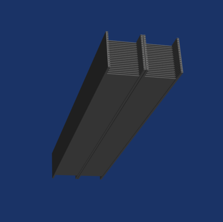
Two fuel element reactor model
The code extract for the building the core is already a little more involved and touches on aspects of the system which will discussed in much more detail in future tutorials (such as Single Assembly tutorial). For now it is not essential to understand every line, but at least to get a feel of how model building is approached.
def build_core():

    from applications.configuration import model
    import core.state
    from material_library.moderators import LightWater

    # this function builds a simple 2 assembly core
    model.facility_description.name = 'ToyReactor'
    model.facility_description.site = 'ToyReactor'
    model.facility_description.unit = 'ToyReactor'
    model.facility_description.type = 'MTR'
    model.facility_description.design_power = 2 * units.MW

    model.state[core.state.fuel_temperature] = 60 * units.degC
    model.state[core.state.moderator_temperature] = 40 * units.degC
    model.state[core.state.moderator_density] = LightWater.density_at(40 * units.degC,
                                                                      1.8 * units.bars)
    model.boundary_condition = boundary_conditions.reflective()

    model.core_map = \
        [[0,    1,  2],
         ['A', _p, _p]]
    model.core_pitches = (7.71 * units.cm, 8.1 * units.cm)

    mft = build_fuel_assembly()  # read mft as `my fuel type`
    mlft = model.inventory_manager.add_loadable_assembly(mft) #read mlft as `my loadable fuel type`
    model.inventory_manager.load_map = \
        [[0,       1,     2],
         ['A',  mlft,  mlft]]

    model.load_map = \
        [[0,      1,    2],
         ['A', 'F1', 'F2']]

    return model
We begin by importing an empty model from the configuration application, and set its basic administrative and
state parameters. The we add the following:
A
core_mapis specified, which defines the positions where core components can be loaded. You will note that nothing is loaded in the core, and a simple placeholder_pis used. The core pitches are also set.We then define two so-called load maps - to load the core with fuel elements:
The first (
model.inventory_manager.load_map), which is a member of the inventory manager class, is populated with a type of fuel. This type of fuel is built by a function calledbuild_fuel_assemblywhich we discuss in the next section. The concept of an inventory manager will also be further discussed in Single assembly tutorial.The second
model.load mapis a map specified with actual assembly names. These will be actual instances (created elements of the given type), for which information such as burn-up or nuclide densities can be stored over time.
Hint
The fact that assembly 'F1' is in the core position where mlft is placed, allows the natural inference that it is of that type.
Input file walk-through - building an assembly
We encountered the function build_fuel_assembly while building the core model. Lets see what it does.
def build_fuel_assembly(ass_name='F1'):

    from ..model import materials
    from material_library.moderators import LightWater
    from core.fuel_assembly import PlateAssembly
    from applications.threading_tools import num_cores

    # This function builds a single plate type fuel assembly,
    # and returns an instance to it
    fa = PlateAssembly(name=ass_name)
    fa.description = 'Test LEU fuel assembly'

    ag3ne = materials.al_clad()
    lwt = LightWater(mass_density=0.9920 * units.g / units.cc)

    fa.number_of_plates = 19
    fa.pitches = 2.95 * units.mm + 1.275 * units.mm  # coolant gap plus plate width
    fa.meat_width = 0.051 * units.cm
    fa.meat_length = 6.30 * units.cm
    fa.meat_height = 59.37 * units.cm
    fa.plate_width = 1.275 * units.mm
    fa.plate_length = 71.68 * units.mm
    fa.plate_height = 625.48 * units.mm

    fa.grid_plate_pitch = 66.8 * units.mm
    fa.slot_insert_depth = 0.5 * (2.74 + 2.59 + 0.45 + 0.55) * units.mm
    fa.slot_insert_width = 1.45 * units.mm
    fa.box = [-0.5 * 75.9 * units.mm, 0.5 * 75.9 * units.mm, -0.5 * 80.15 * units.mm, 0.5 * 80.15 * units.mm]
    fa.axial_region = [-0.5 * 682.9 * units.mm, 0.5 * 682.9 * units.mm]

    fa.clad_material = ag3ne
    fa.grid_material = ag3ne
    fa.moderator_material = lwt

    fa.create_bundle_place_holder()

    fa.complete_universe(material=lwt)
    threads = num_cores()
    tree, stack, new_cells = fa.construct_search_tree(update_archive=False, threads=threads)

    fa.construct_bundle()
    fa.fuel_bundle().depletion_mesh.initial_material_distribution = \
        materials.uranium_silicide(plate_volume=0.051 * 6.30 * 59.37 * units.cc)

    return fa
The assembly build function has a few parts. The first part defines the basic assembly geometry - in this case we use
a macro (method that builds the geometry from a few typical parameters) to build a PlateAssembly. OSCAR-5 contains
a variety of these macros to assist in building typical reactor core components. The result of applying such a macro
is the construction of the fuel element via a set of CSG (Constructive Solid Geometry) objects, which are combined
via various set operations (such as union or intersection). You are of course free to build objects directly
from the available set of underlying primitives.
We will not dwell on each of these macro parameters for the PlateAssembly at this stage, as they are fully described
in Single Assembly tutorial. However, take a look at the parameters and try to imagine how they might relate to the creation of an MTR fuel
assembly as can be seen in your model image.
Note
You will note that all specifications have associated units specified, as OSCAR-5 is unit-aware.
The materials for clad, side-plates and moderator are also defined. You will note that the fuel material
is treated somewhat differently, as it is defined as part of a so-called bundle, as an initial distribution.
In OSCAR-5 burnable components are grouped into bundles, with a particular burnup mesh associated with the
material.
You also note a section in the input file referring to completion of the universe. This is a particular useful feature
which fills the space outside of the constructed geometry with a specified material by building cells iteratively. Without this feature
the user would have to manually define and build these cells, which could be a time-consuming and error-prone task.
We now move on to some step-by-step actions we can perform on this script.
Step-by-step
Let us now use the developed input script, and aim to accomplish the following tasks:
Visualise the model we have prepared.
Generate an input file for use in the Serpent Monte Carlo code to calculate the k-eff of the system.
Run the Serpent calculation.
Post process the results.
We begin by calling the OSCAR-5 system to visualize the prepared geometry. Run the following command:
>>> oscar5 SAFARI_1.projects.demo_simple_integrated_model visualization
Hint
More advanced interactive options exist for viewing and interacting with the geometry, which will be covered in later parts of this tutorial.
Following some mesh processing, a graphical depiction of the assembly should appear, which can be manipulated in space by dragging the mouse.
Next we proceed to generate a Serpent input file for the problem:
>>> oscar5 SAFARI_1.projects.demo_simple_integrated_model --target-mode SERPENT pre --force
Hint
A complete set of available command line options can be requested (at each point in command) by including
--help in the command.
You can inspect the produced input file in the defined working directory, which in this case should be within the projects/DEMO_C1/SERPENT folder. This input file is produced via the Serpent code specific input generation plugin within OSCAR-5.
Next we launch the Serpent calculation, and do so on a separate computational server:
>>> oscar5 SAFARI_1.projects.demo_simple_integrated_model --target-mode SERPENT --config-file neclnx002.cfg execute --force --threads 48
Although this is a Monte Carlo code run, it takes only a few minutes if supplied with enough cores, which is
specified in the command line (in this example 48).
We continue to post process the results:
>>> oscar5 SAFARI_1.projects.demo_simple_integrated_model --target-mode SERPENT --config-file neclnx002.cfg post --force
This command should yield the following output:
keff =   1.52362

Fractional power map:

         1      2
  A 100.00 100.00

Beta Effective                    : 0.00657585 (+- 0.00010942214399999999)
Generation Time                   : 1.94149e-05 second (+- 1.0289897e-08)
Run produced 1 warning(s) and 0 error(s)
Note in this output the reference to warnings and errors. These are written to the system log file, which is located in the top level reactor model folder, named system.log.
Discussion
This simple model combines the input associated with the model building, core loading, and calculational setup. Although putting these elements together is tempting from a simplicity perspective, it could lead to significant duplication if many calculations are associated with a central model, or if many core loadings exist. To circumvent this problem, a distributed modelling approach is used in OSCAR-5, as shown in the table below.
Model Element |
Location |
Description |
|---|---|---|
Component models |
|
Contains a |
Core model |
|
Contains a |
Core loadings |
|
Contains a date-time stamped history of where elements reside |
Calculational options |
|
Contains a py file setting up each calculational option. Some applications have their own dedicated folder. |
In the subsequent parts of this tutorial, we will use the distributed model approach, and demonstrate various calculational applications which are supported by the OSCAR-5 system. Note that in other OSCAR-5 tutorials, some of these applications will be discussed in further detail.