MANAGING YOUR INVENTORY

A critical aspect of reactor analysis is to calculate and track the change in the isotopic inventory of your fuel and other burnable reactor components. This activity is referred to as core-follow. In a core-follow calculation you will simulate the operation of your reactor after the fact, burning your fuel at the same conditions as the plant, and save the updated state of inventory which reflects the new state of the plant.
This chapter explains how to process plant data so that it can be simulated, how to perform core-follow calculations and how to access data from your inventory. The following OSCAR applications are covered in this section:
core-follow
dehomogenization
Initiation
The first thing you need to do with regards to inventory, is to find out where the isotopic inventory for your reactor model is stored. Inventories are stored per assembly, in a folder that is found on the top level of your model space. There can be more than one inventory folder, where one is the official model inventory and the rest are used for studies and ad-hoc analyses. To see which inventory is your official one, you should look in the current core configuration file found at MY_REACTOR/configurations/my_module.py, as discussed in the model navigation chapter.
In this file, look for the following line, in this case stating that the main or official inventory is in a folder called: MY_REACTOR-inventory.
model.inventory_manager.inventory = utilities.path_relative_to(__file__, '../MY_REACTOR-inventory')
Note
The path to inventory can be specified in any application input script too. For instance if you are doing a core-follow calculation, you can specify the inventory in your core-follow input script. OSCAR-5 will then use this path instead of the base one specified in the core configuration file. It is however advised to rather use the base path, so that you can control this path in one place for all the applications and calculations.
Now that you have verified which inventory you are using, the last step in terms of initiation, is to verify if your inventory is up to date. This means that you should check if there is a date entry where isotopic data was written up, at the end of the previous cycle. You can use the manager utility to do this.
oscar5 MY_REACTOR.manager inventory -p *path_to_model*/MY_REACTOR-inventory -t assembly_name
The command above will print all of the time stamps present in assembly_name to your console. If you picked an assembly that was in the core during the previous cycle, you should see the EOC time stamp in this list.
You can also verify if your facility loading is up to date in a similar way.
oscar5 MY_REACTOR.manager facility --data-base my_facility --info
oscar5 MY_REACTOR.manager facility --data-base my_facility --print date_entry
The first command above will print all of the time stamps for entries in your facility loading database to your console. The second command will show the facility loading map at the date entry that you choose from the list of time stamps.
Tip
The manager utility is a very useful tool for quick access to information. It offers a number of ways to interact with your inventory, the rest of which can be explored using the –help option. For example, you can start with the following command and work your way on from there.
oscar5 MY_REACTOR.manager inventory --help
Exploration
There are two main applications related to your existing model’s inventory: Core-follow and ODEHT. Core-follow directly impacts the inventory by updating it, while ODEHT relies on the inventory information—such as number densities—to perform its calculations. These will be explored below.
OSCAR-5 stores large data sets in binary data files. The following data files are relevant to inventory management:
Data File |
Location |
Content |
Updated How |
Updated When |
|---|---|---|---|---|
Official inventory |
inventory/ per assembly |
isotopic number densities, exposure, etc. |
The official inventory is updated every time a relevant application is run in post mode. |
Every core-follow hist save step |
Local inventory |
reload/cycle/, /projects/…/ |
isotopic number densities, exposure, etc. |
A local copy is made of the official inventory any time an application is run, and saved locally. |
Every hist save step. |
HDF5 support for the inventory exploration
The HDF5 extraction capability is aware of typical result objects involved in the inventories.
The inventories can be scanned via:
oscar5 MY_REACTOR.manager hdf5 --scan-path inventory --inventories *path_to_model*\\MY_REACTOR\\MY_REACTOR-inventory --isotopes U-235,Pu-239 --inv-time 2018-01-01
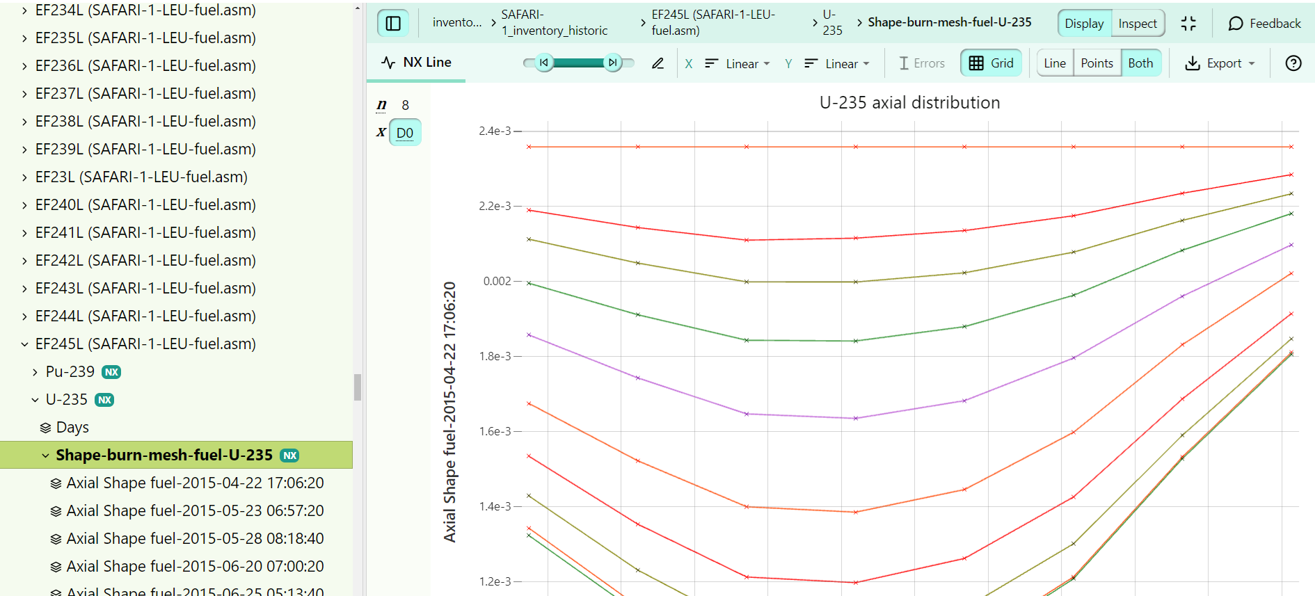
The following data elements are extracted and available for browsing through the HDF5 visualization tool.
Result Objects |
Description |
Available Data Elements |
Comment |
|---|---|---|---|
Burnable component history |
Isotopic evolution of selected isotopes for each burnable component. |
Mass evolution, axial number-density shapes per time-steps. |
Segmented fuel assemblies will present burnup information per region. |
As an example, the following extract shows the U-235 fission cross-section for energy group 6, for each of the off-bases as a function of burnup steps.
Application: Core-follow
The first step for inventory management and core-follow analysis, is to obtain and analyse operational data from your reactor i.e. plant data. This data needs to be processed into a format that can be used by OSCAR-5, as case structures at different state parameters and with various burnup time steps. Once plant data is converted into readable OSCAR-5 data, you can use this to simulate the reactor operation, a procedure referred to as core-follow. The last step is to update your model inventory to reflect the reactor state correctly.
Further information about the core-follow application can be found in the Rapyds documentation under the section on core-follow or multi-step depletion calculations. You can also find a detailed tutorial, covering core-follow calculations, in Full-Core Applications.
Note
The main inventory for your model is stored in OSCAR-5 data structures and remains code-independent. Core-follow calculations however are done with specific simulation codes such as MGRAC or Serpent. These codes use their own formats for inventory and this information is mapped back onto the code-independent main inventory once you post-process the calculations with the post mode.
Core-follow type calculations are typically done in the core_follow/ sub-folder of your model and makes use of data that is typically stored in the plant_data/ sub-folder. You should work through the following steps to perform a core-follow calculation:
Processing plant data.
Plant data format is specific to each reactor. OSCAR-5 supports a number of different formats for plant data, and more can be added as needed. Instructions on how to process your reactor-specific plant data into one of the supported formats should be included in your specific model management document.
Plant data is typically stored under the plant_data/ sub-folder of your model. You should have one data file per cycle.
To access the OSCAR-5 GUI for plant data visualization and processing, the following command is used. The script process_plant_data is found in core_follow/, and can be named anything. Once the GUI is opened, you should open your plant data file from within the GUI, using the navigation bar at the top left.
$ oscar5 MY_REACTOR.core_follow.my_module plant-dataUse of this GUI is extensively covered in the Full-Core Applications tutorial and is not repeated here.
At the end of this step, you will have a data file my_module.pkl that contains a code-independent description of the cycle progression, step-wise and subdivided into “cases” with fixed state conditions and defined time-steps. This data will be read by the core-follow application to create input for specific simulation codes.
Tip
More than one data file can be used to create cycle case data. For instance, if your reactor has an irradiation schedule that is separate from the plant data file, both can be processed and a case structure can be created that represents both of these.
Note
Managing your inventory have been done in a code-independent manner up until this point. You will start defining calculations here and choose simulation codes to run the calculations with.
Creating a new core-follow script.
This is typically done in the core_follow/ sub-folder of your model. You can create a new script here, with for instance the new cycle number as the name. The easiest way of doing this, is copying the script for the previous cycle and modifying it.
For example, you can create a script for your cycle, called my_module, referring to the cycle number for the specific cycle that you will be simulating.
Running a core-follow calculation.
For this discussion we will use the nodal code MGRAC to run core-follow calculations. The following commands should be used. Recall that the –force flag can be added to ensure that all files are recreated and run, even if these already exist.
$ oscar5 MY_REACTOR.core_follow.my_module --target-mode MGRAC execute
$ oscar5 MY_REACTOR.core_follow.my_module --target-mode MGRAC post --show
The execute command will create input for MGRAC and run the MGRAC calculation. The post command will save the updated isotopic states obtained via the core-follow calculation to your model inventory. Results will also be saved to a .res data file. The –show command will display some of the core-follow results for you to inspect.
HDF5 Support for the Core-Follow Exploration
The HDF5 extraction capability is aware of typical result objects involved in core-follow analysis.
The inventories can be scanned via:
oscar5 MY_REACTOR.manager hdf5 --scan-path core_follow --begin-end C1109-1,C1211-1 --exclude test
The following data elements are extracted and available for browsing through the HDF5 visualization tool.
Result Objects |
Description |
Available Data Elements |
Comment |
|---|---|---|---|
Cycle specific res file |
Information extracted per cycle |
Bank positions, critical k-effs, mass maps, total U-235 mass per time-step |
Extracted for each code used for the cycle analysis |
Multi-cycle reactivity |
Set of critical k-effs over all the scanned cycles |
Critical k-effs, cycle markers to identify cycle starts (+ plot markers) |
Overlay red lines indicated each cycle start |
As an example, the following extract shows the U-235 fission cross-section for energy group 6 for each of the off-bases as a function of burnup steps.

Application: ODEHT
It is quite standard to use a nodal code such as MGRAC for computationally intensive applications such as core-follow, to track burnup and manage your inventory. Furthermore, analysis that requires more accuracy / precise heterogeneous geometry, can be done in a code such as MCNP. This means that your inventory data from the homogeneous model needs to be mapped back onto a heterogeneous model.
Extracting and transferring number densities to MCNP is achieved, using the OSCAR De-Homogenization Tool (ODEHT). This application input is contained in the sub-folder MY_REACTOR/odeht. You need a few scripts here that will contain all the information needed to de-homogenize inventory data into a format more widely used i.e. an MCNP number density format. The necessary files are listed and described below:
First, the base ODEHT script that contains instructions on how to export your model compositions from the nodal model created via cOMPoSe, to a text format.
The template file that specifies how data should be written up. This is a cheeta template located in MY_REACTOR/odeht/templates. You can have different templates for different applications, such as one that just dumps the data and one that writes it to specific card formats such as that associated with MCNP input.
The configuration file in MY_REACTOR/odeht/odeht.cfg contains further information particular to MCNP interpretation. This file is typically never changed once set up for your model.
The last file is the data file located in MY_REACTOR/odeht/data/xsdir_mcnp6.1. This file acts like a roadmap to map number density data to ENDF specific formats such as is used in MCNP. This file is never changed.
To run ODEHT and export number densities from your model, you can run the following command:
oscar5 MY_REACTOR.odeht.my_module execute
Note
The ODEHT application takes number densities from the OSCAR-5 nodal model for further use in an existing MCNP model. However, one can also generate an entire complete MCNP input file from the OSCAR-5 model. This can be done for example with the following command:
oscar5 MY_REACTOR.configurations.my_module check-model --target-mode MCNP pre --force
This action will create an MCNP input file in the configurations/my_module folder, under the MCNP folder structure.
Tip
You can choose to get the number density data from MGRAC history files, or from the code independent binary inventory files. The latter option is recommended, since this is usually the primary data carrier for your inventory. After running a core-follow calculation in MGRAC, make sure that the code independent inventory is updated by running the post runmode on the core-follow, for example:
oscar5 MY_REACTOR.core_follow.my_module --target-mode MGRAC post --force
ADAPTATION
Application: Local Inventory branching
Hint
This input example can be found under the projects/demo_inventory_branch.py input file in the SAFARI-1 benchmark
It often happens that you would like to perform a specific calculation at a future time-point, or on a different branched
future which you do not necessarily want to make part of your official inventory. In such a case we can use the so-called
local_inventory_branching application. In this application, a local copy is made of your inventory for which you can specify
the cycle progression. In addition, you can then define a series of further time-steps you would like to include in the cycle progression
for time-points of specific interest where you would like the number densities to be saved to the new local inventory.
You are then free to create new OSCAR-5 applications which can point to this new local inventory, at the time-points of interest, and perform necessary calculations. Lets consider the input you need to provide to this application:
typical input relevant to a most OSCAR-5 applications (working directories, model, cycle name, …)
the new inventory will be created within the specified working directory.
a defined cycle progression in terms of power levels and control rod positions (or searches) as a function of time
a series of additional time-points you would like to include as “save” points in the inventory
In order execute such a calculation, the following command can be used:
oscar5 MY_REACTOR.projects.branch_input --target-mode CODE execute
oscar5 MY_REACTOR.projects.branch_input --target-mode CODE post
Th execute part of the command would run the cycle progression and save the number densities at the requested
time-points to the code-specific inventory. In turn, the post command would update the local code-independent inventory
so that you have it available for further applications.
Multi-inventory management
In this section we explore the mechanisms inside OSCAR-5 to allow the use of simultaneous multiple inventories, in particular in the case where the user is interested in maintaining multiple core-follow lines from different codes, or different levels of fidelity.
This section is still under development.