MANAGING YOUR CORE LOADING

This section describes how an analyst will go about managing and updating the fuel loading in a core, how to design various core loadings and how to assess these from a safety and utilization perspective.

The following OSCAR-5 applications are covered in this section:

facility loading
reload
core design
optimisation

INITIATION

Reactor analysis in support of the day-to-day operations of a facility, can be grouped as tasks on a timeline. The following tasks are done chronologically.

Update your inventory to reflect current state of reactor.

Design a new core reload configuration.

Verify if your new configuration will meet your safety and utilization standards.

Update your model to reflect that this core configuration is indeed the next configuration for your reactor, as opposed to just being a test case.

Once the new cycle is in operation at the reactor, update your inventory accordingly. And repeat.

An accurate representation of the isotopic inventory of your core is needed, before you can proceed to do reload and design type calculations. You are referred to the previous section on Managing your Inventory, for a discussion in this. This section assumes that your inventory is up to date and reflects the current sate of your reactor.

EXPLORATION

There are many applications that have impact on the loading of assemblies and facilities in your reactor model. Applications that are explored in this section includes adding new loadable assemblies to your facility and various ways to design and analyse a new core loading.

Application: Facility loading

Facility loading has to be performed, which places a subset of assemblies into a chosen configuration – normally for your core, but it could of course serve to load elements into other facilities such as the pool, the vault or other storage racks. For this task, you will define a cycle specific script, complete it and execute the script. You can also create different types of loadings, such as actual (as it happened in the core), or design (as you are planning it) to name but two.

More information can be found in Rapyds documentation under the section on facility management.

Firstly, we have to propose a new core layout, and add it to the facility loading data-base. This is done via the facility loading application. The following steps are typically involved:

Create a new facility loading script.

Typically you will have one script per cycle, found in the facility_loading/ sub-folder of your model space. For clarity and consistency, it is recommended to name this script after the upcoming cycle. This facility loading file has one main purpose: to connect a loading date stamp and location to a set of loadable assemblies. These assemblies can include a core layout where each assembly has an assigned place in the reactor, and fresh fuel batches that gets added to a virtual vault, for future use.
Executing this script.
Once you have a facility loading script ready, you can run your application with the following command:
$ oscar5 MY_REACTOR.facility_loading.cycle_name execute
This command will save all defined assemblies to the inventory, and save all specified loadings to the facility loading archive.

HDF5 support for the facility loading exploration

The HDF5 extraction capability is aware of typical results objects involved in facility loading.

The facility loadings can be scanned via:

oscar5 MY_REACTOR.manager hdf5 --scan-path facility --facilities c:\\oscar5\\benchmarks\\MY_REACTOR-facility --isotopes U-235,Pu-239

The following data elements are extracted and available for browsing through the HDF5 visualisation tool.

HDF5 facility loading data elements
Result objects	Description	Available data elements	Comment
Cycle specific facility loading file	Cycle loadings	Fuel loadings per timestep, sub-facility loadings per timestep, isotopic content at loading date	Isotopic content is only extracted if inventory scanning is simultaneously requested. Content is taken from the first selected inventory.

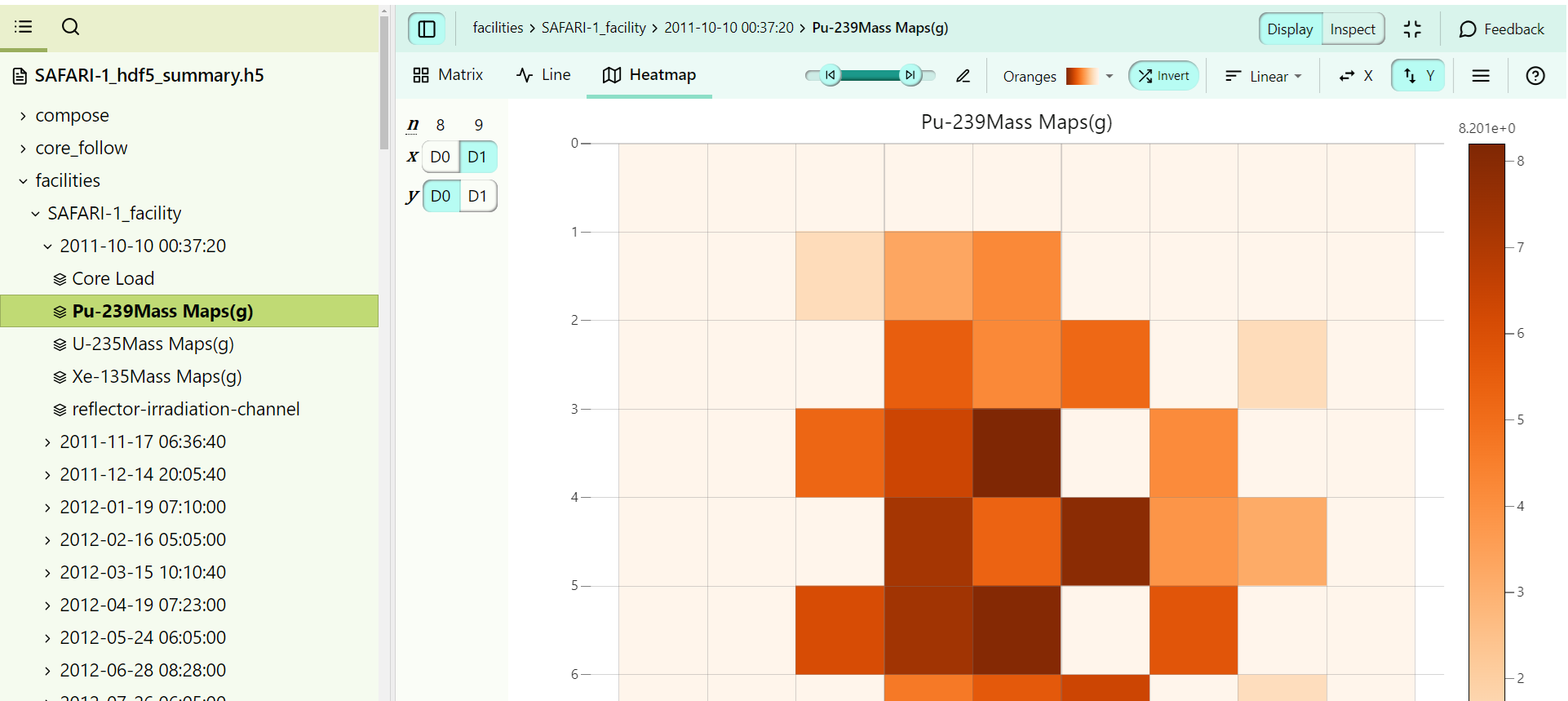
As an example, the following extract shows the Pu-239 mass distribution for the selected core loading timestamp

Application: Reload

Once a proposed core layout has been saved to the facility loading archive, you can proceed to the reload application. This application is used to simulate operation of a cycle that you designed, for the purpose of evaluating safety parameters and utilization performance. Such a reload calculation is typically done prior to accepting a new core design for operation.

Further information about the reload application can be found in the Rapyds documentation under the section on performing reload calculations. You can also find a detailed tutorial, covering core-follow calculations, in Full-Core Applications.

Note

Managing your core loading have been done in a code-independent manner up until this point. Here you will start defining calculations and choose simulation codes to run the calculations with.

Reload type calculations are typically done in the reload/ sub-folder of your model. You should work through the following steps when performing reload calculations:

Creating a new reload script.

This is typically done in the reload/ sub-folder of your model. Here you can create a new script with for instance the new cycle number as the name. The easiest way of doing this, is copying the script for previous cycle over and modifying it.

The typical contents of a reload script includes a description for one or more cycle simulations, using customised operating conditions, at which reload parameters should be calculated. These cycle simulations are referred to as predictive lines. Examples include a snap-shot BOC calculation at hot conditions and a cycle burnup to a planned EOC date. Next, a set of results to be extracted from the simulations is defined, such as time-dependent bank positions, as well as potential results to calculate from the extracted parameters, such as shut-down margin and EOC fuel mass.

Your typical reload script will also contain some information needed for writing up a reload report, such as required content, title and list of authors, to name a few. Since a lot of this information is quite generic and static for all reload reports, the bulk of the reporting parameters can be stored in a separate script that is simply called for each cycle. You should have such a “generic” report skeleton under MY_REACTOR/reload/report_template and at MY_REACTOR/reload/generic_report.py in your model.

Running a reload calculation.
The following commands need to be executed in order. Here we are using a new cycle script called my_module_reload found under the reload/ sub-folder in your model. The first two commands (prediction) runs the predictive lines in the nodal code MGRAC (it is the user’s choice which code to use), and updates results in the local directory created for this cycle reload. The next command cases runs any additional calculations required in order to calculate results from the simulations, at specified core state and time (from predictive lines). The fourth command runs a post-processing of your reload calculations, extracts predefined results and performs any predefined calculations with the these results. The last two commands are used to create a reload report.
>>> oscar5 MY_REACTOR.reload.my_module prediction --target-mode MGRAC execute
>>> oscar5 MY_REACTOR.reload.my_module prediction --target-mode MGRAC post
>>> oscar5 MY_REACTOR.reload.my_module cases --target-mode MGRAC execute
>>> oscar5 MY_REACTOR.reload.my_module --target-mode MGRAC post
Executing these last two commands will generate the report in rst (restructured text) format, and build a pdf and html reload report. Your reports can be found under MY_REACTOR/reload/my_module/report/build/ in the latex (for pdf) html sub-folders.
>>> oscar5 MY_REACTOR.reload.my_module --target-mode MGRAC prepare-report
>>> oscar5 MY_REACTOR.reload.my_module --target-mode MGRAC build-report

Hint

With somewhat more advanced input options, different prediction and cases calculations can be run with a variety of different codes in one reload application.

Application: Core design

As a natural extension to the core reload application, we find in addition the core design application, which aims to allow multiple core designs to be proposed, consecutively run, and then compared. However, this application is at present implemented as a decentralised application in the model space for users who require this functionality, and is in the process of being centralised as a general OSCAR-5 application. This process is however not yet complete and this section will be updated in future once this is done.

Application: Reload optimization

Hint

This input example can be found under the design/demo_optimization.py input file in the SAFARI-1 benchmark

Reactor core loading optimisation, or the search for an optimal set of fuel placements in reactor core positions in the upcoming reactor cycle (or set of future cycles) is an important aspect around reload design. Research reactors in particular can face the challenge of having many areas of core performance which requires an element of optimization, given the multi-purpose nature of such machines. In the case of RRs, it is then quite important to employ truly multi-objective solution schemes, which do not aim to yield a single optimal loading, but rather present a so-called Pareto-front of best possible trade-off solutions for the set of multi-objective requirements.

The first important step to performing a reload optimisation analysis for a given reactor core is to establish a good understanding and associated numerical representation of the major objectives under consideration when loading the core. When engaging the reload engineer on such matters, an extensive amount of information is typically supplied which envelopes both the constraints to which the core must adhere (from a safety and utilisation perspective) and the objectives which are to be maximised, minimised or targeted to define a good core. It very often happens that the considerations related to objectives and constraints overlap, and care must be taken to address these subtleties and extract the correct interpretation.

General approach in OSCAR-5

In OSCAR-5, we consider the multi-objective Harmony Search optimisation scheme as preferred algorithm, as past research has shown its natural applicability to the core reload design problem. Some special features around this implementation in OSCAR-5 include:

A code-independent framework for core optimisation, meaning that different physics solvers can be utilised in unison, for the sake of calculating the required values.
Optimisation can be performed for any loadable parts of the reactor grid, including non-fuel components, control rods, reflectors or irradiation positions.
Multi-zoning for the placement of loadable components is supported, to facilitate guidance of the optimisation algorithm, by defining preferred sub-regions for components with specified properties.
A generalised model is developed for selecting which loadable components in the inventory should be considered eligible for loading.
Results selected for defining constraints and objectives can be combined, scaled and adjusted to form more intelligent optimisation quantities, relevant to the reactor under consideration.

To achieve this goal in OSCAR-5, we use the application termed multi-objective. There are four steps involved in this process:

Define your optimization zones and set of available assemblies in each.
Define your set of objectives and constraints.
Associate each objective or constraints with a calculable quantity in OSCAR-5.
Perform the optimization calculation and analyse the result.

We will discuss each of these in the upcoming sections.

Define the optimization zones and assemblies

We begin by segmenting the core into regions within which a defined set of assemblies maybe placed by optimization mechanism. As an example, we consider a possible zoning for the SAFARI-1 core, as depicted in the following figure.

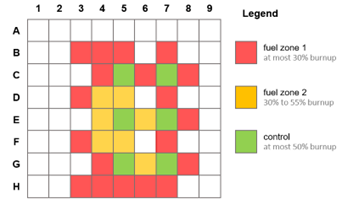
To accomplish this, we first define a zoning map:

loader = CoreLoader()

loader.template_map = \
[[0,    1,   2,        3,        4,         5,        6,       7,        8,     9],
 ['A',  _,   _,        _,        _,         _,        _,       _,        _,     _],
 ['B',  _,   _,        1,        1,         1,        _,       1,        _,     _],
 ['C',  _,   _,        _,        1,         3,        1,       3,        1,     _],
 ['D',  _,   _,        1,        2,         2,        _,       1,        _,     _],
 ['E',  _,   _,        _,        2,         3,        2,       3,        1,     _],
 ['F',  _,   _,        1,        2,         2,        _,       1,        _,     _],
 ['G',  _,   _,        _,        1,         3,        2,       3,        1,     _],
 ['H',  _,   _,        1,        1,         1,        1,       1,        _,     _]]

Thereafter we select an inventory to use, and further choose assemblies from the inventory which could be candidates for each zone:

loader.provider = utilities.path_relative_to(__file__, '..','SAFARI_1_inventory'), '10-10-2011 00:37:20'
# all assemblies with at most 15% burnup in the center ring
loader.set_candidates(1, name_predicate=lambda n: re.match(r'EF\d+L', n),
                      predicate=lambda asm: asm.get_mass('U-235') > 0.70 * 340 * units.g)

# rest of fuel assemblies 15% to 55% burnup
loader.set_candidates(2, name_predicate=lambda n: re.match(r'EF\d+L', n),
                      predicate=lambda asm: (1.0-0.55) * 340 * units.g < asm.get_mass('U-235') <= 0.70 * 340 * units.g)
# control with less than 55% burnup
loader.set_candidates(3, name_predicate=lambda n: re.match(r'C\d+L', n),
                      predicate=lambda asm: (1.0-0.50) * 223 * units.g < asm.get_mass('U-235'))

Defining objectives and constraints

Now to choose the goal of the optimization. As illustration, the following could for example represent a set of objectives and constraints relevant to a core optimization

Example of objectives for reload optimization
Goal	Objective	Numerical representation
Maximise	Minimum thermal flux in all irradiation positions	Minimum thermal flux in all in-core irradiation positions over the active height
Minimise	Discharge U-235 mass of 3 fuel elements	Sum of the mass of the three lowest mass fuel elements at EOC
Minimise	Discharge U-235 mass of 3 fuel elements	Sum of the mass of the three lowest mass fuel elements at EOC

Example of constraints for reload optimization
Type	Constraint	Numerical representation
Inequality	The core power peaking factor must be below the safety limit	Maximum local hotspot heat-flux-based peaking factor < 3.5 at BOC
Inequality	Start-up bank must be more than 50% extracted	BOC critical control bank insertion depth > 50% extracted at BOC

As an illustration of how OSCAR-5 can be used to represent these, we define, firstly for the startup bank constraint:

startup_bank = f.calculate(cc.critical_position(state=state.xenon(0.0),
                                                bank_names=['control', 'regulating'],
                                                search_banks=['control', 'regulating'],
                                                target_keff=target_keff,
                                                bank_positions=fixed_banks,
                                                parameters={'bank_search.continue_on_failure': True,
                                                            'max_feedback_iteration': 30,
                                                            'power': model.facility_description.design_power}),
                           transform=lambda x: float(x[1]),
                           default=0.0)

# start up bank must be more than 50% extracted
f.add_greater_than_constraint(startup_bank, 50.0)

Here we can note two steps. The first defines an intended constraint variable named startup_bank to an OSCAR-5 output token (or result) named critical_position. This critical_position is one of the standard results from the critical_case (named here cc) application in OSCAR-5 which is used to calculate a snapshot neutronic state of the reactor.

The second step defines the full constraint statement, and requires that the startup_bank must be greater than 50%.

As further illustration, we also include the definition of one of the objectives, and consider in particular the maximization of thermal flux in irradiation positions. Note here that we include a position filter map to make sure only fluxes from irradiation positions are considered.

position_flt = \
     [[0,  1, 2, 3, 4, 5, 6, 7, 8, 9],
     ['A', _, _, _, _, _, _, _, _, _],
     ['B', _, _, _, _, _, 1, _, 1, _],
     ['C', _, _, 1, _, _, _, _, _, _],
     ['D', _, _, _, _, _, 1, _, 1, _],
     ['E', _, _, 1, _, _, _, _, _, _],
     ['F', _, _, _, _, _, 1, _, 1, _],
     ['G', _, _, 1, _, _, _, _, _, _],
     ['H', _, _, _, _, _, _, _, _, _]]

irr_position_thermal_fluxes = f.calculate(cc.ChannelFlux(attr='thermal_flux_map',flt=position_flt, bank_positions=fixed_banks,
                                                                          parameters={'power': model.facility_description.design_power}),
                                                                          transform=lambda x: x.min()[0])

f.add_objective_to_maximize(irr_position_thermal_fluxes, tag='Min Irr Pos Thermal Fluxes(Flux)')

These definitions of course contain many further aspects to explain, and more information can be found in relevant benchmark examples and OSCAR-5 documentation.

Perform the optimization calculation

The optimization calculation of course requires many additional input parameters to set, such as specific setup options for the harmony search algorithm, an possible initial population to seed the algorithm with initial core designs to consider (optional) and various detailed problem specification options.

However, once the input file is fully developed, it can be called via (in this case setting default code to MGRAC, although individual calculations can be passed to other codes from the input file):

oscar5 MY_REACTOR.design.optim_input --target-mode MGRAC execute
oscar5 MY_REACTOR.design.optim_input --target-mode MGRAC post
oscar5 MY_REACTOR.design.optim_input --target-mode MGRAC post --show

These steps would execute the optimization calculation (running a number of samples in order to search the space), post processes the results, and generating the GUI designed for exploring the results.

As an indication of the typical output, see the following figure which illustrates the typical Pareto front, which is the set of multi-dimensional non-dominated points from which the decision makers can choose a solution to implement.

These user can then select one of the points on the left-hand side, and the corresponding core loading which resulted in that set of objective values will be displayed on the right-hand side.

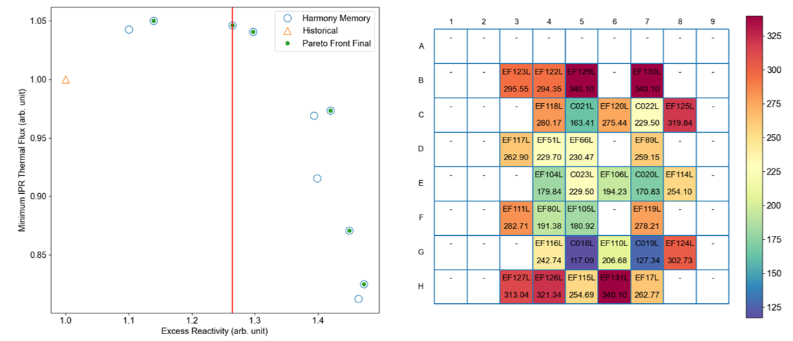
It should be clear that for a two-dimensional optimization problem, this representation is sufficient to see the value of all objectives contributing to a specific loading. If the problem dimension is higher than two dimensional, the graph above has options for plotting various combinations of two objectives at a time. However, in order to see all objective function values for a given point on the pareto front, an additional visualisation option. This additional visualization is illustrated below.

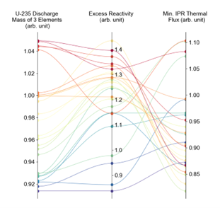
In this figure (for a postulated case of three dimensions) it becomes much easier for decision makers to select an optimal point from the pareto front which meets their business needs.

It should be reiterated that the outcome of the optimization of core reload is a core reload design, indicating which fuel elements are loaded into which positions. It is still incumbent upon the reload designer to pass this proposed core through the full reload analysis process, in order to extensively check that the proposed core indeed meets all core safety and utilization requirements.

ADAPTATION

As mentioned earlier as a hint, it is possible to customize your reload analysis to use multiple codes, so that the most appropriate code can be used for any given output parameter. In this section we illustrate how this form of reload application refinement can be done.

Hint

This input example can be found under the design/demo_mult_code_core_analysis.py input file in the SAFARI-1 benchmark

Multi-code core analysis is helpful when parameters of different levels of detail are to be combined in a single report. This occurs, for example, often in core reload analysis. The example script demonstrates how a reload script can be adapted to combine nodal analysis for global parameters, with fine scale flux assessments with Monte Carlo codes. This is done via passing a specific parameter pack to each calculational call, as highlighted below:

sss2_param = {'target_mode': 'SERPENT',
              'particles': 64000,
              'source_iteration': 50,
              'max_iteration': 500,
              'threads': 96,
              'config_file': 'C:\\Users\\rianp\\Desktop\\Repos\\Modelling_project\\neclnx002.cfg'}

mcnp_param = {'target_mode': 'MCNP',
              'particles': 64000,
              'source_iteration': 50,
              'max_iteration': 500,
              'threads': 96,
              'config_file': 'C:\\oscar5\\client_models\\daffodil_mcnp.cfg'}

b_eff = parameters.calculate(cs.beta_effective(parameters=mcnp_param.copy()),
                             reactivity,
                             0,
                             calculation_group='Limits')


mx = parameters.calculate(cs.maximum_power_density(mesh=(6, 60), parameters=peaking_param),
                          reactivity,
                          0,
                          calculation_group='Power')

This extract indicates how a parameter pack can be defined for both MCNP and Serpent 2, followed by calculational requests to calculate the b-eff with MCNP and the maximum power density with Serpent 2 in a single reload script. Please review the full script to gain a better understanding of how various parameters can be customized.