NAVIGATING YOUR OSCAR-5 MODEL

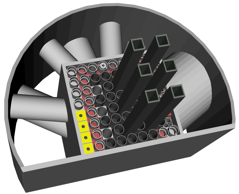
The term “OSCAR-5 model” refers to the entire data model for your reactor together with all calculations done with this data model. This entire work space is stored in one parent folder which is usually named after the reactor that you are modelling. This chapter will show you how to navigate through your OSCAR-5 model.

Initiation

Your OSCAR-5 model will typically be stored in a central place where multiple users can access it, such as a local or cloud server with version control. Depending on available storage space, only specific parts of the model might be stored. You may need to initiate your model once checked out, or it might be stored in a working state and up to the current state of your reactor (i.e. with the current inventory). This model state and how to initiate it, is usually described in a model management report that can accompany your model, typically found at docs/model_management/html/index.html in your model space.

Since model initiation is model specific, it is not discussed further here.

Exploration

In this section we will discuss various ways in which to explore and gain insight into your OSCAR-5 model. We will start with reviewing the geometric setup of the reactor, followed by the nodalization and creation of a nodal model (if used). We will also take a brief look at the automated model documentation options in OSCAR-5.

OSCAR-5 stores various data sets in binary data files. The following data files are relevant to overall model management. Further details around the update and management of these data carriers will be provided in the application specific sections later in this training manual.

**Data carriers related to model management**
Data File	Location	Content	Updated How	Updated When
Assembly archives (.asm)	model/	The `asm` archives contain a description of the material and geometric layout of a given reactor core component. The archive further includes various representations of this model, including some mesh representations which could be useful for certain codes/applications. Both the heterogeneous and homogeneous model representations are stored in this archive.	Archiving a model	Any time `archive` is run, when the `cOMPoSe` model is deployed, or when `exposure` calculations are performed.
Nodal configuration (.nfg)	model/	The nodal configuration file contains the nodal (homogenized) representation of all non-loadable (static) components of the reactor core.	Deploying a nodal core configuration through `cOMPoSe`.	Any time deploy is run in `cOMPoSe`.
Facility loading	top level	The facility loading database contains a time-stamped representation of the loadable components in a given loadable facility. The typical example of this would be placement of fuel elements in the reactor core for every operating cycle, captured at the date of core loading.	Updating facility loading.	Any time facility loading is run.
Official inventory (typically a folder named MY_REACTOR-inventory)	top level	Detailed exposure and isotopic number density distribution in a burnable component.	Running OSCAR-5 applications which performs either depletion or activation analysis.	Every step in the calculation for which an inventory update is requested.
General `res` objects	Application working directory	Varied content depending on the application, but typically related to results calculated.	Running an application in `post` mode (processing code specific output files and writing up the code-independent res file.	Ad hoc.

Mechanism for model exploration

OSCAR-5 input is generally captured in the form of simplified Python scripts. The execution of these scripts typically results in some action performed, and some resulting data carrier or database updated. These data carriers in the OSCAR-5 models can be explored in a number of ways. Primary approaches include:

Using the built-in visualisation methods associated with running the scripts.
Using the built-in --show options associated with selected application modes. This typically would open a small dedicated Graphical User Interface (GUI) element to browse the results just obtained with an application.
Using the rapyds API (Application Programming Interface) to open the results files directly in python.
Using the OSCAR-5 manager utility to scan an OSCAR model (or model component), and generating an HDF5 database summarizing the most important information in all data carriers. Such an Hierarchical Data Format (HDF5) database can then be browsed with any HDF5 compatible viewer.

The OSCAR-5 manager HDF5 mode

The OSCAR-5 data carriers are not directly browsable. However, it is often useful to get an overview of the current state of the model, and quickly navigate through the most important data elements and outputs in order to investigate specific issues. In this instance, the OSCAR-5 manager is a useful tool, and in particular the HDF5 database generator which can then be easily browsed.

HDF5 (Hierarchical Database Format v5) is a hierarchical database structure which largely functions like a Windows folder structure, but where the leaves at the end of the branches are multi-dimensional datasets. Once such a database is generated, a variety of viewers are available to browse and plot the content. One of the nicer options in this regard is the so-called H5Web interface. As such, we recommend using the free browser tool myHDF5. You can go to https://myhdf5.hdfgroup.org/ and load the HDF5 file that you have produced (normally named *.h5) to start exploring and visualizing data. From here you can also export any of this data to .csv format. Other Python-aware systems, such as Jupyter notebooks or VSCode have so-called H5Web extensions to view HDF5 files.

Throughout this tutorial we will provide support to help you to apply the HDF5 generation mechanism to the relevant sections. However, in general, the entire model can be scanned and packaged into an HDF5 database via:

oscar5 MY_REACTOR.manager hdf5 --force

Note

Note that the –force option will over-write the existing HDF5 file if found. You can control the name and path of the HDF5 file using the –hdf_file option.

Hint

oscar5 calls always need to be made from one-step above the top-level reactor directory.

This approach will, by default, aim to scan your inventories, facilities, compose area, core-follow area, reload area and project area. However, this can take a significant time and create a large HDF5 file, therefore it is recommended to rather scan selected areas separately.

You can control the areas (folders in your top-level model) which you want to scan for example, via:

oscar5 MY_REACTOR.manager hdf5 --scan-path facility,inventory

which will then only scan the model for facility loadings and inventories, and update these sections in an existing HDF5 file.

Note

If an existing HDF5 file is found and –force is not specified, the selected scanned areas will be over-written, but others retained. In this way you can maintain a single integrated HDF5 database for your model for easy perusal.

A number of filters are available to control the content of the HDF5 database:

**Manager HDF5 mode control options**
Command Line Option	Description	Example	Comment
–scan-path	List the subset of top level areas in the model to scan.	–scan-path core_follow,projects,verification	All folders in the selected spaces will be scanned, and relevant file types will be read recursively.
–inventories	List the subset of inventories (full path) to scan.	–inventories c:\oscar5\benchmarks\MY_REACTOR\MY_REACTOR-inventory	Multiple inventories can be specified as comma delimited.
–facilities	List the subset of inventories (full path) to scan.	–facilities c:\oscar5\benchmarks\MY_REACTOR\MY_REACTOR-facility	Multiple inventories can be specified as comma delimited. If an inventory is also read, the first inventory will be used to populate mass maps at start of cycle in the facility area (for all selected isotopes).
–isotopes	List the isotopes for which detailed information should be extracted.	–isotopes U-235,Pu-239,Xe-135	Additional isotopes extend the time of extraction.
–begin-end	Start and end cycle for core-follow and reload scan extraction.	–begin-end C2101,C2111	Core-follow and reload result extraction specific, and core-follow results will be automatically compared to reload predictions for the same cycles.
–inv-time	Inventory data extraction can be time consuming, and as such an initial time stamp can be specified from which information. is extracted.	–inv-time 2021-01-24	The time will be applied to all inventories, and will inadvertently limit the BOC mass maps extracted as part of facility loading processing.
–compare	Select an alternative .h5 file to compare to. All common datasets between the new and comparator databases will be compared in terms of percentage difference.	–compare test.h5	Multiple comparison data sets can be supplied in comma delimited form.
–replace	Advanced option to allow cross comparison between datasets with different names between the new .h5 file and comparator sets.	–replace replacements.yaml	The yaml file contains a set of keywords per area to make replacements with. Names in the new .h5 file are replaced in order to match them to names in the comparator database for comparison.
–exclude	Advanced option to ignore cycle names containing a particular piece of subtext.	–replace replacements.yaml	The yaml file contains a set of keywords per area to make replacements with. Names in the new .h5 file are replaced in order to match them to names in the comparator database for comparison.

After the database is generated, it can be opened via the H5Web interface. The viewer has a number of built-in multi-dimensional visualization options associated with 1D, 2D and multi-dimensional datasets. As an example, the figure below shows a typical .h5 file for a reactor model in the H5Web interface. Note that for each dataset, multiple views are available, and that most datasets have a preferred data representation which is coded into meta-data of the dataset via the so-called NeXus extensions to HDF5 visualization (https://manual.nexusformat.org/user_manual.html )

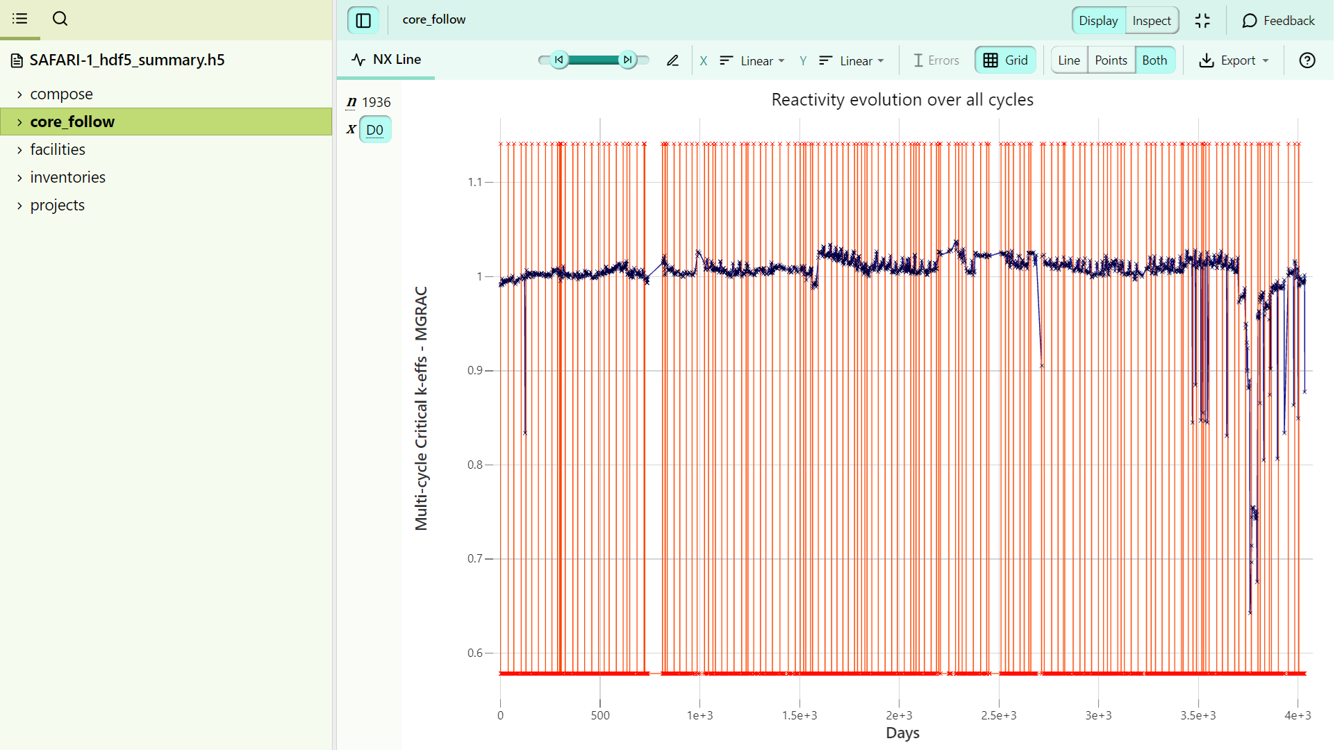
The data extracted, and associated visualization options via this approach, are discussed in more detail in each of the relevant application sections in this manual.

Hint

As an overall example of an HDF5 model representation, you can inspect the example provided with the SAFARI-1 benchmark model, named Demo_SAFARI_1_hdf5_summary.h5 in the SAFARI_1 top level directory.

Code-independent heterogeneous model

One of the strengths of the OSCAR-5 platform, is the concept of a code independent heterogeneous reactor model. This concepts enables the user to build a detailed model of their reactor without having to consider any code specific inputs / restrictions. This code independent model can be built and undergo quality checks and then be ready for later use, knowing that the reactor description is correct and complete.

In this section we will learn a few ways in which to explore the code independent heterogeneous model. The first approach is to view a plot of the code independent model components, as follows:

See what the reactor looks like.

View the core configuration file found in the configurations/ sub-folder of your model space (called MY_REACTOR for the remainder of this training document).
You can run the following command for the configuration file assumed here to be my_configuration.py
oscar5 MY_REACTOR.configurations.my_configuration visualization --interactive --parts
From this plot, you can see how the reactor core and pool look at a glance. For further information you can inspect the configuration file my_module.py. You can obtain information here such as the core layout, grid pitches, and some generic reactor information.

See what the assemblies look like.

From the configuration file above, you can determine what types of assemblies are loaded into particular core positions. Next you can view these assemblies.
You can run the following command for assembly my_component.py, which is located in the model/ sub-folder of your OSCAR-5 reactor model.
oscar5 MY_REACTOR.model.my_component visualization --interactive
From this plot you can see an assembly at a glance. For further information you can inspect the model input file my_module.py. You can obtain information here on the geometric and material composition of the assembly.

See how the reactor is loaded.

The configuration file only describes a generic, time-independent setup. To see information on the cycle-specific data, such as the core loading with associated fuel and control assemblies, you have to go to the facility loading files found in the facility_loading/ sub-folder.
You can run the following command for any cycle’s facility loading my_module.py, which is located in the facility_loading/ sub-folder of your set. However this will not give you much more information than you got by viewing the configuration, since assembly names are not included in the plot.
oscar5 MY_REACTOR.facility_loading.my_module visualization
For further information you can inspect the facility loading file my_module.py, to see information such as the core layout at a specific time stamp.

Up to now you have viewed models using the built in OSCAR visualization tool. You can also use Serpent or MCNP plotters in much the same way, to view 2D cuts of your configuration and models. An example is given here, for a 2D image of a fuel assembly viewed along the xy-plane, at the axial centre of the assembly.

oscar5 MY_REACTOR.model.fuel_assembly plotter --z --executable 'path to Serpent'

This command will set up a Serpent input file of the model, call Serpent to make a plot, and save the image in a sub-folder in your model directory.

Note

There are many options to use with the plotter. To see all your options, type:

oscar5 MY_REACTOR.model.fuel_assembly plotter --help

At this point you should have all of the information needed to understand how your heterogeneous model looks. Further, you should be ready to run calculations in codes such as the Monte Carlo codes MCNP or Serpent, which can use the heterogeneous model description as is. However, if you want to use a nodal diffusion solver such as MGRAC, you may want to investigate how your model is nodalized into homogeneous zones / nodes. This is covered in the next section.

Homogenized nodal model

The OSCAR-5 platform offers a powerful tool for the homogenization of your reactor model, in preparation for use with the MGRAC nodal diffusion code. The standard approach in OSCAR-5 is to model all non-fuel components in their exact core environment and to generate their nodal data from one or more 2D full core heterogeneous Serpent calculations. Fuel and other loadable components (such as control and irradiation assemblies) are modelled in an approximate but representative environment.

This homogenization procedure will be explored next, under the compose/ sub-folder of your system. Again we will inspect a plot of the homogenized reactor model first, followed by reviewing the Python scripts and lastly the existing documentation and to investigate the errors introduced in the model during the homogenization procedure.

Inspect components to be homogenized.

View the loadable components such as a fuel assembly (for this example found at model/my_module.py)
You can run the following command to visualize the assembly my_component and the nodal grid over which this assembly will be homogenized.
oscar5 MY_REACTOR.compose.my_component visualization
Hint

In the viewer, toggle the component transparencies to better see the homogenization grid.

Inspect the whole reactor to be homogenized.

View the core model (my_homogenized_model.py) with a homogenization grid overlay.
You can run the following command for this visualization:
oscar5 MY_REACTOR.compose.my_homogenized_model visualization

HDF5 support for the cOMPoSe model

The HDF5 extraction capability is aware of typical result objects involved in the cross-section generation process.

The compose can be scanned via:

oscar5 MY_REACTOR.manager hdf5 --scan-path compose --isotopes U-235,Pu-239

The following data elements are extracted and available for browsing through the HDF5 visualization tool.

**HDF5 cOMPoSe model data elements**
Result Objects	Description	Available Data Elements	Comment
Snapshot cross-section sets	Generated static cross-sections via lattice codes connected to the OSCAR-5 platform	Multiplications factor, multi-group flux distributions, power distribution	These are the same as standard results extracted from any critical case application
Lattice burn lines	Results associated with each burn line performed (per lattice cut) associated with a homogenization calculation	k-inf evolution, isotopic evolution (for selected isotopes) over time	Extracted isotopes are taken from the isotope set specified in the HDF5 filter
Lattice off-base	Off-base cross-sections at each burnup step	Macro and micro cross-sections as a function of off-base and energy group (trending and detailed)	Subset of cross-sections currently extracted - to be further expanded. Micro-scopic cross-sections for selected isotopes.
2D equivalence, 3D test results	Critical case results for each of these tests	Multiplications factor, multi-group flux distributions, power distribution	Results provided for both the homogenized and lattice codes.

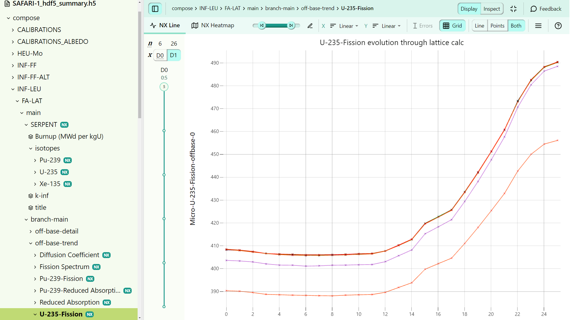
As an example, the following extract shows the U-235 fission cross-section for energy group 6 (lowest energy group in a 6-group model) for each of the off-bases as a function of burnup steps.

Auto-generated model documentation

In this section we discuss two specific options available in OSCAR-5. The first relates to how you can go about attaching a report to any given application, and customize the content of the report. In addition the process of dynamically connecting output variables from any given application to the report is explained. The second documentation option discussed is the process of auto-documenting your model itself, and using options such as FreeCad interfacing to support and enhance the model documentation.

This section is still under development.

Adaptation

In this section we illustrate a few examples of introducing model changes and options in your OSCAR-5 model. This includes simple adaptations, like updating particular geometry or material specifications associated with existing model components, adding new model components or updating the overall core configuration. The section defines the required data carriers which have to be updated for each of these cases, and how to go about it.

This section is still under development.