Step-by-Step

In this chapter you will build your mini core reactor and run a few calculations with your models. There are many ways in which a model can be build, depending on how you interpret the engineering specifications and how accurate you want to model your components and reactor. This tutorial includes numerous example inputs for the reactor you will build. You will learn how to build your own models, using the OSCAR-5 user guide, model description documents and the provided examples to guide you.

Getting Started: The OSCAR-5 Setup for this Scenario

In order to proceed with this tutorial, OSCAR-5 should be installed on your system. The project space for this tutorial can be found at

<TutorialPath>/MINI_CORE.

Please note that <TutorialPath> is the path to your OSCAR-5 Tutorial Series and is typically (but does not have to be) set to ~/oscar5_tutorials/, where ~ refers to your home directory. This model can also be found on GitLab.

The actual calculational codes within the OSCAR-5 system should of course be pre-installed and their paths defined within the OSCAR-5 configuration files.

The commands shown in the steps below are often illustrative and do not have to be run again. This will be indicated where appropriate. Unless you are working in PyCharm, make sure that the virtual environment is activated in the terminal you are working, by typing

>>> conda activate oscar5

Hint

In the step-by-step that comes, you do not have to execute all commands (you can of course), but at typically only perform that defined as a “Todo”.

Step 1: Becoming Familiar with Basic Commands

In the previous tutorial, First OSCAR-5 Run tutorial, you looked at several Python input scripts that fulfilled different functions in building and using a reactor model. These scripts were already finished, with all the Python coding done for you, and the focus was on how to use them. In this section we will step away from fully formed scripts to have a look at the constructs inside them, and become familiar with the underlying functionality of OSCAR-5. To this end we will play around without the need to first create all the project infrastructure associated with a full models as seen in the First OSCAR-5 Run tutorial. This will help you to understand the input files that appear later on in the tutorial.

Python provides an interactive interpreter session where you can directly see the effect of your input, which we will now use. An interpreter is the machinery that translates your input into instructions that the underlying system understands. The Python interpreter is a great way to learn about the interface, to quickly check the effect of your input and to get online help.

To access the interpreter, click on the Python Console tab in PyCharm. You can read more on using the Python interpreter and learn some Python basics in the OSCAR-5 user guide, under A Quick Introduction to the Python Interface.

Material specifications

Material specification forms a critical part of any analysis system. OSCAR-5 provides functionality to specify material data required for neutronics calculations as well as additional data required by other systems such as thermal hydraulics.

There are many ways in which to define materials in OSCAR-5 and as such it might be best to start with a practical example. We will define the material specifications for the LEU uranium silicide meat. We will use the definition as in the SAFARI-1 benchmark description, repeated in the table below for convenience.

In order to create a routine to define this material, let us look in detail at the following input. This will define the uranium silicide meat material specification. We will need to access the core package, which contains all fundamental system functionality in the OSCAR-5 system. The two modules in this package that we will use are the material module to define and manipulate isotopes and material mixtures of isotopes, and the units module, to define physical dimensions and units. Thus we will import both of these modules from the core package. We will also define the mass and volume of the fuel meat, and calculate its density. This is needed in order to define the material using mass fractions (as per table).

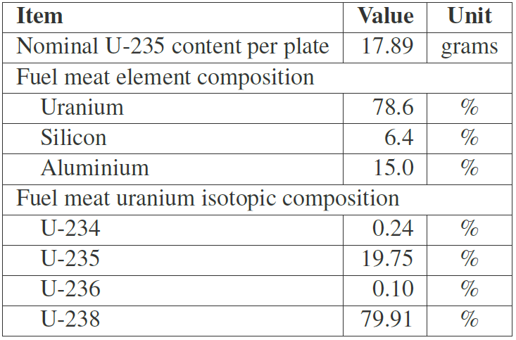
Material specifications for uranium silicide

The density is calculated with the formula:

dens = mass/(fraction of U-235)/volume

where mass and enrichment is given in the specifications table and the plate volume is calculated from the specifications in the benchmark document. After you have defined the density, you can see what the value is by typing :py:’dens’ and pressing enter.

>>> from core import material
>>> from core import units
>>> mass = 17.89 * units.g
>>> plate_vol = 6.3*0.051*59.37 * units.cc
>>> dens = mass / (0.785 * 0.1975) / plate_vol

Now we will define the material composition in terms of mass fractions by using the utility called MaterialMassFractionMixer , which requires the material density we just defined. From the example below you can see that isotopes are added to the mixture in terms of mass fractions.

>>> mixer = material.MaterialMassFractionMixer(dens, total=100.0)
>>> mixer.add('U-234', 0.24*0.786)
>>> mixer.add('U-235', 19.75*0.786)
>>> mixer.add('U-236', 0.10*0.786)
>>> mixer.add('U-238', 79.91*0.786)
>>> mixer.add('Si', 6.4)
>>> mixer.add('Al-27',15.0)

Thereafter a number of meta data can also be specified such as name, color and type.

>>> m = mixer.mix()
>>> m.name = 'meat'
>>> m.type = material.tags.fuel

Finally, we can look at the composition of the material we have defined in terms of both the mass fractions and number densities:

>>> print(m)

which gives the following output:

Material     : meat
Type         : fuel
Mass density : 6.0492 g/cc
Isotope Wt Nd (1/b/cm)
Al-27   15.00   %   2.02522e-02
Si-Nat  6.40    %   8.30112e-03
U-234   0.19    %   2.93622e-05
U-235   15.52   %   2.40595e-03
U-236   786.0   ppm 1.21304e-05
U-238   62.81   %   9.61171e-03
Total   100.00      4.06124e-02

Todo

Open the Python interpreter by clicking on the Python Console tab in PyCharm and enter the above example for the meat specifications. Print the material definition to your screen and compare the output to the input from specifications table.

One more quick example to look at is how to use the numerous pre-defined materials that can be found in the material_library package. This package contains modules such as moderators , structural , gasses , etc. Let us access the built-in material for water in two different ways, using the two synonyms the system provides for the same built-in material. These synonyms are equivalent, and can be used in exactly the same way. In your Python interpreter you can type:

>>> from material_library.moderators import LightWater
>>> from core import units
>>> lwt = LightWater(pressure=1.8*units.bar, temperature=20*units.degC)
>>> print(lwt)

Or, if you know the density, you can type:

>>> from material_library.moderators import H2O
>>> from core import units
>>> water = H2O(mass_density=0.9928*units.g/units.cc)
>>> print(water)

The above examples show just a few ways in which to define material specifications. Please consult the OSCAR-5 user guide for the complete user documentation and further examples. In particular you can browse to Building Assembly Libraries Building Assembly Libraries (click on this title in the left pane table of contents and go to Data Model), and go to the section on Specifying Materials.

Hint

The user documentation is the best place to seek help or clarification, but you can also use the Python interpreter for this. For instance, once you have imported reflectors module from the material_library package, you can type help(material_library.reflectors) to see which built-in reflectors are available. Just remember that you must import a module before you can access it.

Now that you have some basic knowledge, we can have a look at the material specifications for this tutorial. Standard practice is to create a separate file for all material specifications (as is done in this tutorial), but if you wish you can also include the specifications in the individual component modules. All necessary materials for this tutorial have already been defined and you can browse this model/materials.py file by clicking on it in the PyCharm project tree view.

Todo

Open materials.py and have a look at the different materials specified. Compare the input to the material definitions given in the Material Library section of the model documentation. The same information can be found in SAFARI-1 benchmark document, specifically in Table 2 (Section 4.2), Table 3 (Section 4.3) and Table 5 (Section 5.1) of the benchmark document.

The Constructive Solid Geometry package

Before we continue, we take some time to become acquainted with the tools OSCAR-5 provides to simplify the specification of the geometry in your model. As in the previous section, we will use the Python interpreter. More information on the extensive geometry processing capabilities can be found in the OSCAR-5 user guide, under the Constructive Solid Geometry (CSG) package. You can again access the interpreter from within PyCharm or the terminal. The most basic constructs available are called primitive regions, and are a part of the in the primitives module of the csg package.

Let us build a few simple objects. In your Python interpreter, type:

>>> from csg import primitives
>>> from core import units
>>> ball = primitives.Sphere(radius=10*units.cm)
>>> block = primitives.Cube(radius=10*units.cm)
>>> rectangle = primitives.RectangularCylinder(width=5*units.cm, length=10*units.cm)

The sphere and cube are bounded in all three dimensions, while the rectangle is unbounded in height. Each geometry object contains the show() method to visualize it. You can look at the objects you have built by typing for example ball.show() in the interpreter. Additional constructs are also contained in the region_macros module. These are mostly extensions of the primitive regions. Let us look at a cross and a pipe as examples.

>>> from csg import region_macros
>>> cross = region_macros.square_cross(radius=12*units.cm, width=2.5*units.cm)
>>> tube = region_macros.pipe(diameter=12*units.cm, width=0.25*units.cm)

In the case of the pipe, the first argument is the outer diameter, while the second is the thickness of the wall.

All of the above geometry objects are created in some Cartesian coordinate system, and the object is centred on the origin by default. Unless otherwise specified, infinite objects are aligned along the z-axis. They may then be placed at a specific location in the space by adding a position argument, or aligned along a different axis by specifying it, when they are constructed. For instance, to build a ball with its centre at (30;30;30), type:

>>> ball2 = primitives.Sphere(radius=10*units.cm, center=(30*units.cm,30*units.cm,30*units.cm))

and to build a rod aligned along the x-axis, type:

>>> tube2 = region_macros.pipe(diameter=12*units.cm, width=0.25*units.cm, alignment=primitives.ALIGNMENT.X_AXIS)

Alternatively, objects may me moved or rotated by applying one of the many transformations the system allows. To move the ball we initially constructed without a position argument (and therefore by default located at the origin) we use the add_transformation method, which is defined in the geometry module of the core package, and needs to be imported first. The transformation we will use is a simple translation to move the centre of the ball to (-10;-10;10).

>>> from core import geometry
>>> ball.add_transformation(geometry.translation(-10*units.cm,-10*units.cm,10*units.cm))

After all of this, we now have two balls of the same size with their centres located at (30;30;30) and (-10;-10;10), respectively. The show() method will not show any change, because it centres on the object being viewed.

In the same way that objects can be translated, they can also be rotated around an arbitrary vector or by using Euler operations, and transformations can be combined. Below, we will simply rotate the cube through 45º around the vertical axis.

>>> block.add_transformation(geometry.rotation_around_vector(45*units.degrees, vector=[0,0,1]))

Viewing the block after the above transformation is shown in the following figure. Note that transformations accumulate, i.e. they are combined when executed one after another.

Todo

Follow along with the commands above in the Python interpreter. Combine different transformations of the objects you created above to see how they build on each other.

The geometry objects you have built up to now can also be combined to build more complex constructs by using regularizing set operations, i.e. complement, intersection and union, which are indicated by ~, & and |, respectively. For instance, we can make an object that consists of a combination of the ball and the block.

>>> region = ball | block
>>> region.show()

Note the effect of the earlier transformations of these regions, as can be seen in the figure.

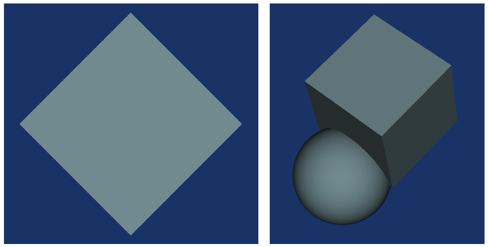
Cube rotated through 45º around the vertical axis (left), and union of the transformed cube and sphere (right)

Let us look at a more practical example. To make a pipe with a length of 10 centimetres, we can cut the tube we built above, by defining planes that bound it at the top and bottom.

>>> top = primitives.Pz(position=5*units.cm)
>>> bottom = primitives.Pz(position=-5*units.cm)
>>> pipe = tube & top & ~bottom
>>> pipe.show()

The first line creates a plane perpendicular to the z-axis 5 cm above the origin along the z-axis. The second line creates a similar plane 5 cm below the origin. The third line states that the pipe must include the tube, as well as the region bounded by the top plane, but outside the region bounded by the bottom plane. More interesting constructs can be created by combining transformations and regularizing set operations.

Todo

Using available primitive regions and regularizing set operations, build a block with two holes of different diameter through it.

Step 2: Creating a project space for your reactor

Now that you are comfortable with interacting with Python, let us return to regular input scripts that can be saved. You can now close the Python interpreter, and click on the Terminal tab in PyCharm.

In the previous tutorial, First OSCAR-5 Run, the project space was already there, and you essentially interacted with an existing model. When modelling a reactor from scratch, however, the very first step is to create a project space in which all your OSCAR-5 material for this reactor (such as model input, output and calculational applications, etc.) will be placed. The project space for this reactor has already been created and numerous example inputs are included here. This section will therefore discuss how to create a project space, but you will not actually run the commands given here.

Under <OSCAR5Path>/rapyds there is a script called setup_reactor.py. The purpose of this utility is to create a project space for a new reactor model. This is the only utility that you would normally need to access directly from within your OSCAR-5 installation space. The project space is a set of mostly empty sub folders and some useful modules, providing you with a starting place to work in. Let us see what you can do with this script. In your PyCharm terminal, go to <OSCAR5Path>/rapyds.

To see which options are available to you, type:

>>> python setup_reactor.py --help

Please note that you should not actually run this script in this tutorial, since the project space has already been created for you. However, if you wanted to create a new project space, the command would have been something like this:

>>> python setup_reactor.py MINI_CORE --parent ~/oscar5_tutorials/ --description "Mini core tutorial"

The parent directory will change to where you want to create the reactor space called MINI_CORE.

Todo

You can now go and browse this project space, since the rest of this tutorial happens here: <TutorialPath>/MINI_CORE. For simplicity, directory structures will hereafter be referred to by omitting the first part of the file path.

Step 3: Building an Assembly Archive for the Fuel Assembly

Now that you have a project space to work in, you are ready to start creating the models. The first step in the OSCAR-5 approach is to create code independent core components. Since we have defined our materials and understand how to specify basic geometry elements, we are ready to model the reactor components. A good place to start is the fuel assembly, because this represents the most important component in your reactor. In this section you will build a plate-type fuel assembly from scratch. A number of example inputs are also provided in this tutorial, with two examples for the fuel assembly:

• model/fuel_simplified.py is a “bare bones” model with only the PlateAssembly macro and cylinders to represent the top and bottom structure of the assembly, and

• the model/fuel_detailed.py is more of a “state of the art” model that includes an accurate representation of the adapters as well as grooves in the side plate extensions to top and bottom, and plate combs above and below the fuel plates. This detailed model was used in the full core configuration, and is therefore the model that will be used for any calculations done with the model.

You can browse these sample input files but do not get lost in the detail, focus only on the build part for now.

Creating a skeleton input file

When you create a project space, you automatically create another helper utility to take note of, known as the manager. This utility can be used to write template modules for a variety of assembly types, as well as template inputs for several standard applications. In order to see what you can do with this script, you can type

>>> oscar5 MINI_CORE.manager --help

in the embedded PyCharm terminal.

Note that you can always use the --help mode when running any OSCAR-5 command if you want to get more information. For instance, if you want more information specifically on the assembly command, then you can type:

>>> oscar5 MINI_CORE.manager assembly --help

Now we want to create a template file for the fuel assembly using the manager.py script, which you can do this by typing:

>>> oscar5 MINI_CORE.manager assembly --base-name MINI_CORE_LEU_fuel --description "SAFARI-1 LEU fuel assembly" fuel_assembly

This command has already been executed for you, which created the template file called fuel_assembly.py in the MINI_CORE/model directory, where all component models are placed. The name that you will use to refer to this assembly in the rest of your OSCAR-5 model is MINI_CORE_LEU_fuel. At this point you have selected to create a generic assembly, which you will soon change to a fuel assembly.

Note

It is important to understand that this tutorial will only guide you in this process and that there are many different ways in which to construct models, which you will learn as you build experience with using the system.

You will create a model for the fuel assembly from this skeleton script, so let us have a look at it:

"""
SAFARI-1 LEU fuel assembly
==========================

Sources
-------
Detailed description of all sources

Assumptions and Simplifications
-------------------------------
What simplification and/or assumptions were made during component modeling

Version Log
-----------
- 1.0.0 : Initial model definition
"""
from core import *
from csg import *
from . import materials

def build(*args, **kwargs):
    fa = Assembly(name='MINI_CORE_LEU_fuel')
    fa.description = 'SAFARI-1 LEU fuel assembly'
    # =========================================================
    # Set some QA parameters
    fa.__source__ = 'Short list of data sources'
    fa.__version__ = '1.0.0'
    fa.__author__ = ''
    # =========================================================
    # Define assembly structure (add cells)

    return fa

if __name__ == '__main__':
    from applications.assembly_archiver import main
    main(source=build)

You will notice that this template has the layout of a typical Python script and contains four parts listed from top to bottom:

• A comment header which is used for auto generated documentation;

• a preamble with all import statements;

• a body where the application parameters are set; and

• a closing section detailing how the script will be executed.

Some general import statements are given in the template, and you can edit them to fit your specific needs. In this case the parts of the system that we will need to add to the imports are the built-in moderators from the material_library module, as well as the materials module that is part of this reactor model. There are several ways to do this, one of which is shown below:

import material_library.moderators
import materials

Todo

Look at the options options available to construct an assembly template using the --help mode of the manager utility, as shown above. Thereafter, you can open the template input file provided, MINI_CORE/model/fuel_assembly.py. See where the --base-name, --base-cls and --discription arguments are used. Finally, add the necessary additional import statements.

Creating a plate-type fuel assembly box

Let us look at the body of the input file, the build method. The first step is to change our assembly class from generic to a plate-type fuel assembly, called PlateAssembly. To do this, edit the provided file as follows:

def build(*args, **kwargs):
    fa = Assembly(name='MINI_CORE_LEU_fuel')

    fa.number_of_plates = 'SET ME'
    fa.pitches = 'SET ME'
    ...

By default, the manager creates an input with the Assembly class. One of the steps in making this an input for a plate type fuel assembly is to change that to fuel_assembly.PlateAssembly. Detailed documentation on the PlateAssembly class, which is a member of fuel_assembly inside the core module, can be found in the OSCAR-5 user guide under Building Assembly Libraries and the subsection Plate fuel assembly. This class is a macro that you can use to specify all parameters of a plate-type fuel assembly box (i.e. the plates and side plates of the assembly). This is done in the form of a list of parameters that collectively encompass all the information needed to fully define the section of the fuel assembly containing the plates (the structures above and below the plates are built separately). This list can be divided into sections that each describe a particular aspect of the fuel plate assembly, and is described in detail below. See the following figures for clarification of the parameters.

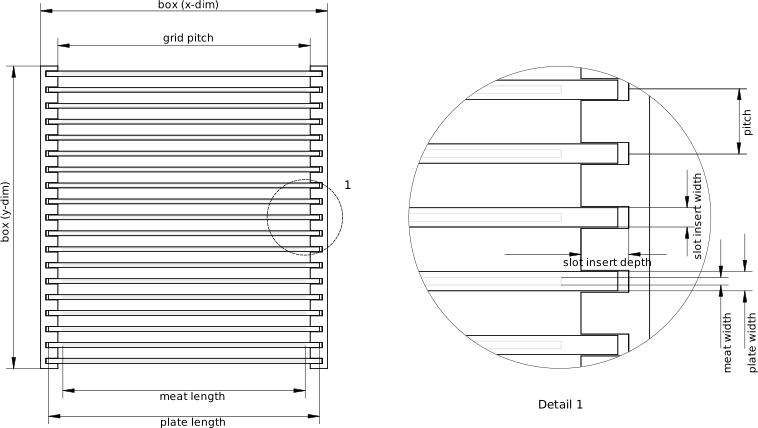
Radial schematic illustration of the PlateAssembly structure

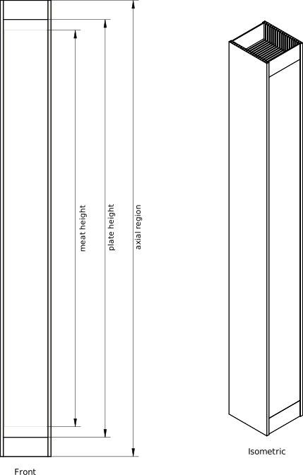
Axial schematic illustration of the PlateAssembly structure

Values for all of these parameters for the fuel assembly under consideration can be found in or inferred from data in the specifications for the SAFARI-1 fuel with simplified geometry, found in the OSCAR-5 model description for this tutorial (Tutorial found here), when you open model_description.html on top-level and is repeated in the table below for your convenience. Note that all parameters with a distance dimension can be either a single value, in which case it is deemed to be the same for all instances of the repeating structure, or a list of values that contains an entry for each instance of the structure.

Fuel plate lattice specification

Parameter	Description
number_of_plates	the number of fuel plates in the lattice
pitches	distance between centre point of plates, i.e. the sum of the gap and plate width
plate_width	total width (or thickness) of a fuel plate, including all meat and cladding layers
plate_length	total length of fuel plates, including sections without meat
plate_height	total height of fuel plates, including sections without meat
meat_width	width of the fuel meat, i.e. fissionable material
meat_length	length of the fuel meat
meat_height	active height of the core
grid_plate_pitch	distance between grid plates, also known as side plates
slot_insert_depth	depth to which the plate extends into the groove in the side plate
slot_insert_width	width of the groove in the side plate into which the fuel plate extends
box	radial area containing plates, including structures deemed as side plates
axial_region	axial region of the grid, in most cases this is the axial region occupied by the plates
orientation	the direction in which the plates are oriented, i.e. horizontally or vertically
centre	defines the location of the centre point of the plate lattice relative to the coordinate system used to construct the rest of the assembly
clad_material	material assigned to all cells deemed to be cladding
grid_material	material assigned to all cells deemed to be part of the side plates
moderator_material	material with which all areas between plates are filled

In the sample inputs you will see that some parameters are given as little equations rather than numbers. This useful Python feature allows you to only use data obtained from engineering specifications, so that when others read your input they can immediately see which parameters you have used and trace it back to the source data.

Hint

Instead of thinking of your input as a static recipe, rather use it as a worksheet containing all your calculations, comments and other useful bits of data. This is a powerful feature of using Python input because it allows for better traceability and repeatability of your input.

The PlateAssembly macro automatically builds all the cells needed to construct the detailed geometry of the fuel plates and associated structure. By necessity, this involves a large number of cells, which are computationally expensive whenever intersections between cells are searched for. OSCAR-5 provides a mechanism to avoid doing so unnecessarily. You will see in the example file, fuel_simplified.py, that the PlateAssembly parameters are followed by

fa.create_bundle_place_holder()
# Add water around the assembly box
fa.add_cell(fa.axial_region & ~fa.box,
    material=fa.moderator_material,
    description='Water around assembly box')

This adds water around the plate bundle and reserves the space that it would occupy with a single cell. Inserting create_bundle_place_holder is not necessary, but it is recommended since it cuts back severely on the calculational time needed to check intersections of cells when using archive later on, especially when using OSCAR-5’s functionality to automatically fill empty cells with water.

Todo

In your assembly input file (model/fuel_assembly.py), change your Assembly to PlateAssembly and add all parameters that describe your fuel geometry and material distribution as described in the specifications table, such as number_of_plates, plate_width, etc. You can view the specifications in the section Plate bundle and view the CAD drawings in the section Drawing Sheets. Continue by reserving the volume that will be occupied by the PlateAssembly with a single cell, and surrounding this with water.

Adding the adapters

You are almost done, but the PlateAssembly macro alone does not describe the whole fuel assembly. You still have to add the top and bottom structures and fill the rest of the assembly environment (or universe) with water. We will be using the csg (constructive solid geometry) package to define the rest of the fuel element.

You can have a look at the two example fuel elements included in this tutorial. In the fuel_simplified.py file the top and bottom adapters are simply modelled as cylinders attached to the PlateAssembly box. This is done by defining some primitives (cylinders and planes in this case) and adding the regions bounded by these primitives to the fuel assembly model by using region_macros and add_cell.

In the fuel_detailed.py file the adapters closely match those in the benchmark specification, by using the RectangleToCircleAdapter class from the build_adapter method. A detailed example of such an adapter is given in the OSCAR-5 user guide in the subsection on Adapters under Building Assembly Libraries.

You can visualise these two adapter models using the visualization command as follows (you do not need to run the archive command first, as these example models have been pre-run for you):

>>> oscar5 MINI_CORE.model.fuel_detailed visualization --interactive

and

>>> oscar5 MINI_CORE.model.fuel_simplified visualization --interactive

We will follow the example of the simplified fuel assembly. An extract that covers the specification of the top adapter is shown below:

# End adapters
# Primitives
height_box = 682.9 * units.mm
length_adapt = 57.0 * units.mm + 63.5 * units.mm + 19.25 * units.mm
top_adap = region_macros.axial_strip(lower=0.5 * height_box,
        upper=0.5 * height_box +
        length_adapt)
rad_out = Cylinder(radius=0.5 * 70.55 * units.mm)
rad_in = Cylinder(radius=0.5 * 63.50 * units.mm)
# Top adapter cells
fa.add_cell(rad_out & ~rad_in & top_adap,
     material=materials.al_ag3ne(),
        description='Top adapter',
        part='TopAdapter')
fa.add_cell(rad_in & top_adap,
        material=fa.moderator_material,
        description='Water hole in top adapter')
fa.add_cell(~rad_out & top_adap,
        material=fa.moderator_material,
        description='Water outside top adapter')

You can see that primitives are used to define regions, which are then added to cells along with the material with which to fill that cell, a description and a part. Assigning cells to a part makes the CAD files created with the model documentation much easier to work with.

Todo

Define the top and bottom structures. You can use as much or as little detail as you wish to represent the adapters.

Filling the empty spaces and specifying burnable regions

After the rest of the structure, such as adapters, has been defined, the next step in completing your core component is to fill the remaining parts of the model with water, using complete_universe to do so. Once this is done, the space reserved with create_bundle_place_holder can be filled with the actual cells from the PlateAssembly macro with construct_bundle . You could, of course, have placed the construct_bundle command anywhere after completing the PlateAssembly and omitted create_bundle_place_holder , but it is much more efficient to do it this way by only filling the placeholder with the complex set of cells of the assembly plates after using complete_universe. Doing so cuts back severely on the calculational time needed to check intersections of cells when using archive.

Hint

You could also leave out all the water cells in your input, since complete_universe will fill them for you. In fact, it could also be passed as an argument to archive on the command line as –complete-universe. This is often the preferred approach when debugging your model.

Finally, the space that contains burnable material, in this case fuel, must be identified and filled with the appropriate burnable material. The following extract shows how to finish your model by filling the empty cells with water and specifying the burnable regions:

    # Fill model with water
    fa.complete_universe(material=fa.moderator_material)

    # Construct the bundle (i.e. add all the plates)
    fa.construct_bundle()

    # Initiate the fuel material
    fa.fuel_bundle().depletion_mesh.initial_material_distribution = materials.fuel_leu(plate_volume=0.51*units.mm * 63.00*units.mm * 593.7*units.mm)

    return fa

if __name__ == '__main__':
    from applications.assembly_archiver import main
    main(source=build, world_box=(7.71*units.cm, 8.1*units.cm))

The fuel_bundle manages materials that can be depleted or activated. It acts like a material exposure mesh and can be customized without modifying the geometry.

Hint

The world_box is mainly used to clip the space for visualization purposes. If it is omitted, the assembly is clipped when it is placed in the core to fill the space available there.

Your fuel assembly model is finally complete, and you can visualize it in an interactive threedimensional viewer. To do this, type:

>>> oscar5 MINI_CORE.model.fuel_assembly archive --search-tree --force
>>> oscar5 MINI_CORE.model.fuel_assembly visualization --interactive

You can inspect your assembly by rotating, zooming and hiding certain materials to see sections otherwise hidden. Later in this section you will also be shown how to export your model to FreeCAD, where you can peruse it further by viewing cuts through the model and making accurate measurements of the components.

Todo

Fill any empty spaces in your model with water, then replace the space reserved for the fuel assembly box with the cells built by the PlateAssembly . Finally, set the initial material for the depletion mesh define the volume that surrounds the assembly for your fuel assembly, then run archive and visualization to inspect your final model.

Step 4: Building Archives for the other Assemblies

The control assembly

Congratulations on building your very first core component! The fuel assembly was discussed in a lot of detail which hopefully helped you to gain some confidence in navigating the OSCAR-5 user guide and interpreting the contents of given example inputs.

Next we will look at the control assembly for our mini core. It is a follower type control, with a cadmium absorber coupled to a fuel follower. The fuel follower section is constructed in a similar way to the plate type fuel assembly box from the previous section. What is different from the fuel assembly is that the fuel section is connected to a cadmium absorber section through a coupling piece, the whole assembly is surrounded by an aluminium sheath, and the whole assembly is movable axially. Care must therefore be taken to correctly align the control assembly, which is movable and longer than the other assemblies, axially with the core.

We will not go into quite as much detail here as we did for the fuel assembly, and you do not have to build an assembly of your own. The control assembly for your reactor has already been built and you can find it at model/control_assembly.py. You can browse this model by clicking on the file in your PyCharm project tree view.

We will now take a look at the input for this model and discuss some specific features for a control assembly. If you had to create this model from scratch, you could have used the manager.py utility and typed something like:

>>> oscar5 MINI_CORE.manager assembly control_assembly --base-name MINI_CORE_control --base-cls Assembly --desription "SAFARI-1 follower control assembly"

This would once again have created a generic assembly, which you would have to change to the appropriate assembly type in the build section of the input file. We will use the FollowerPlateAssembly macro to model the MTR type fuel follower control rod. This macro simply combines the PlateAssembly (which we used for the fuel assembly) and the ControlAssembly types. The ControlAssembly class models any assembly that moves in order to control reactivity, and is found in the core.control module. You can find a list of all parameters associated with this macro in the OSCAR-5 user guide on Generic assembly and Follower type plate assembly.

We will look at some of the important parameters for the ControlAssembly class.

If you open the control_assembly.py input file in PyCharm you will see that the first part of the file looks much like that of the fuel assembly, with a comment block for auto documentation at the top, followed by the import statements.

Note that the FollowerPlateAssembly is imported, but not ControlAssembly . This is because FollowerPlateAssembly inherits the parameters of the ControlAssembly class. Also note the parameters regarding the movement of the control rod that is imported.

This is followed by the build() method, as with the fuel assembly, and the fuel follower parameters using the same macro format as used previous sections. The follower type fuel differs from the standard fuel in a number of ways, however, the same parameters must be set, only with different values in this instance. The macro does not allow for any structural parts around the fuel box, parallel to the plates (i.e. perpendicular to the side plates), and these must be added separately. This part of the follower assembly is added in the section commented as # Structure around fuel box.

• Thereafter all outstanding geometry is added using region_macros and add_cell, similar to how the cylindrical adapters were added to the simplified fuel assembly example. These include the structure around the fuel box (as discussed above), the coupling piece, top and bottom structures and the absorber part of the assembly.

• The initial material for the depletion mesh is then defined (again, similar as in Section 2.3).

• The control parameters are set, using the ControlAssembly class. These parameters are shown in the excerpt.

• Lastly again a closing section detailing how the script will be executed.

# ======================
# Set control placement and movement data
cr.base_position = fully_extracted() # Current position
cr.travel_direction = up() # Extraction direction
cr.total_travel_distance = 74.79 * units.cm # Total travel in length units

Hint

The visualization command will show what is in the current assembly archive, regardless of what changes have been made to the input script. Therefore, you must use archive before visualization for new assembly models, or whenever you want to view the effect of changes you have made.

Todo

Familiarize yourself with the provided model for the control assembly by using the visualization command to inspect the geometry. View this model in conjunction with the SAFARI-1 follower control assembly description in the auto generated model documentation.

Irradiation target

The core contains a grid position that is available for experiments or isotope irradiation, commonly known as a rig. For the purpose of this tutorial, the position will be used to irradiate a cobalt cylinder with a diameter of 5 cm and a height of 10 cm. This irradiation target will be inserted into a holder assembly, known as a rig, before being loaded into the core. The irradiation target is modelled separately from the rig assembly. They will only be combined when the target is inserted into the rig at load time, which is usually for a specific application. The model of the target is therefore relatively simple, and has already been created for you. The file in question is model/irradiation_sample.py. As before, to crate a skeleton input file, one would have used the manager.py as follows:

>>> oscar5 MINI_CORE.manager assembly irradiation_sample --base-name MINI_CORE_irradiation_sample --base-cls Assembly --description "Irradiation sample that will be placed in the rig assembly"

Todo

Archive and view the sample. Look at the model and the material specification. Note the unbounded nature of this model, and identify the command used to fill all regions not specified with water.

Irradiation rig

The next step in modelling the cobalt irradiation experiment is to design a rig into which the target can be loaded to keep it in position. In this example the rig consists of a simple cylinder with top and bottom adapters similar to the fuel assembly. If you had to create this model from scratch, you could have used the manager.py utility and typed something like:

>>> oscar5 MINI_CORE.manager assembly rig_assembly --base-name MINI_CORE_rig --base-cls Assembly --description "Irradiation sample holder rig assembly"

This assembly differs from those that came before in that it may or may not contain another component. We refer to any structure that has this property as a loadable facility. To make the rig assembly a loadable facility, the following lines are included towards the end of the file:

#========================================================
# Central water channel / loadable facility
rig.add_facility('irradiation-channel', state=lwt)
rig.add_cell(axial & inner, facility='irradiation-channel')

The first line after the comments indicates that this assembly contains a facility, names the facility and sets the default state of the facility as filled with light water. An assembly may contain multiple facilities, as long as they have unique names and do not overlap. The second line after the comments assigns the cells that belong to the facility.

Todo

Open the file and inspect it, visualize the model and compare to its description in the model documentation.

Structures outside the core

The region outside the core that forms part of the model is dealt with in a similar way as assemblies. It is viewed as a single component with at least one loadable facility that will contain the core once all the parts of the model are assembled. The pool in this example contains an aluminium core box that surrounds the space where the core will be placed, as well as a beryllium reflector outside the core box on the North side of the core. The script that describes the pool structure is located at

<TutorialPath>/MINI_CORE/model/pool_facility.py.

The core box extends to 10 cm above and below the end adapters, while the beryllium block lies next to the fuel plates axially, but does not line up with the core grid radially. Structures that go into the pool may be described in the pool component script, or in separate scripts that are then used in the pool construction script. We will show an example of each; the core box and beryllium block will be built directly inside pool_facility.py, while the grid plate with slots into which core components are anchored will be constructed in grid_plate.py in the same directory. Let us start with the grid plate, as this needs to be complete before we can use in the construction of the rest of the pool.

Grid plate

If you had to create this model from scratch, you could have used the manager.py utility as before, but in this instance the base class would be Pool instead of Assembly:

>>> oscar5 MINI_CORE.manager assembly pool_facility --base-name MINI_CORE_pool --base-cls Pool --description "Pool facility with beryllium reflector"

Let us first discuss the grid plate, shown in the figure below, as this needs to be complete before we can use it in the construction of the rest of the pool.

The grid plate with slots for assemblies and space for control rod to pass through

This is the first build script where we will make use of repeated structures and we will use some Python scripting to make this easier. In our model there are only two types of grid plate slots: one for fuel and the irradiation facility, with a round slot in the aluminium plate for the nozzle, and one with a whole assembly sized rectangular hole punched from the aluminium plate for the control element. We will only construct the cells for one of each type and then pack them next to each other in the necessary order by translating instances of them in space. Let us start by looking at the methods used to build each one. If you open the file grid_plate.py, the first method that you will encounter after the import statements is fuel_slot(target, x_min, x_max, y_min, y_max). Note that this method receives arguments, which determine the dimensions and position of a given slot. A similar method for the control slot follows thereafter.

The two methods for building the cells for a single slot are called from inside the build() method inside a loop, in fact we use two nested loops, to go over every row, and every column position in that row, as shown in this excerpt:

for c in range(1,4):
    for d in range(1,4):
        if c==d==2:
            control_slot(grid, new_x, new_x + x_pitch,
            new_y, new_y + y_pitch, ’core’)
        else:
            fuel_slot(grid, new_x, new_x + x_pitch,
            new_y, new_y + y_pitch, ’core’)
            new_x = new_x + x_pitch

    new_y = new_y + y_pitch
    new_x = x_anchor

Todo

Look at the fuel_slot and control_slot methods and make sure you understand how the parameters passed to them are determined in each iteration. How would calling them individually differ from the above loop?

Pool, core box and beryllium

Now that we have completed the grid plate that will form a part of the pool, let us have a look at pool_facility.py. Note that the grid_plate is now amongst the import statements:

from core.pool import Pool
from csg import *
import materials
from material_library.moderators import LightWater
import grid_plate

The pool is also considered a loadable facility, because the core will be placed inside it at a later stage. In the build() method, cells for the beryllium and the core box are added in the same way as for any other assembly, and they are therefore fixed in place. After these fixed components have been built, the grid plate is inserted and a placeholder is defined for the cells that will be filled by the core.

# Insert the grid plate
pool.add_cells(*grid_plate.build().structure)

# ==============================================================
# Flag placement of core within pool
pool.core_cell = Cell(box_inner & model_upper_bound &
    ~primitives.Pz(grid_plate.core_grid_top),
    material = LightWater(mass_density = hot_dens),
    description = 'Core')
pool.core_center = (0 * units.cm, 0 * units.cm, 0 * units.cm)

The pool usually extends to the outer edges of the boundary, and as such, this is the place where we can declare what lies beyond these boundaries. Additionally, the core and pool generally have different states. These are set in the following manner:

# ====================================================
# Define cells outside model boundary
pool.add_cell(~model_radial_bound,
    material=LightWater(mass_density = cold_dens),
    outside=True)
# ====================================================
# Specify pool state, which is distinct from core state
pool.set_state(state.moderator_temperature(25 * units.degC),
    state.moderator_density(cold_dens))
# -----------------------------------------------------
# Add water around the core box
# Fill model with water
pool.complete_universe(material=LightWater(mass_density = cold_dens))

Todo

Visualize the pool and connect each part to the place in the script where it was defined or imported.

Step 5: Building a Core Configuration

Now we have a full set of reactor components! It is finally time to define your core configuration. The core configuration for your reactor has already been built and you can find it at configurations/core_config.py. You can browse this model by clicking on the file in your PyCharm project tree view. The following figure shows a view of this core configuration.

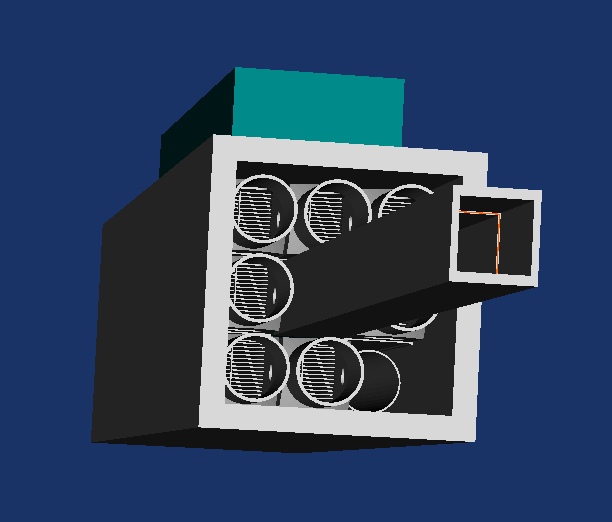
The mini core reactor model

If you had to create this model from scratch, you could have again used the manager.py utility and typed something like:

>>> oscar5 MINI_CORE.manager configuration core_config --desription "Core configuration for Mini Core design"

This would have created a generic configuration file core_config.py for you to populate according to your design. This has already been done and you can view this model. The command for this is much the same as for an assembly. You can type:

>>> oscar5 MINI_CORE.configurations.core_config visualization --interactive

Lets look at the core configuration module in more detail. This file is repeated here for your convenience. You will benefit from referring to the OSCAR-5 user guide while we browse the file. In particular you can look under Building Core Configurations and the subsection on Building the model.

from applications.configuration import *
from core import *
from ..model import assemblies
# ----------------------
# Facility meta data
model.facility_description.name = 'MINI_CORE'
model.facility_description.site = 'MINI_CORE'
model.facility_description.unit = 'MINI_CORE'
model.facility_description.type = 'MTR'
model.facility_description.design_power = 5.0 * units.MW
# ----------------------
# Set core map
ir = assemblies.MINI_CORE_rig()
model.core_map = \
[[ 0, 1, 2, 3],
 ['A', _p, _p, _p],
 ['B', _p, _p, _p],
 ['C', _p, _p, ir]]
# ----------------------
# Set core pitches
model.core_pitches = (7.71 * units.cm, 8.1 * units.cm)
# ----------------------
# Loadable assembly layout
fa = model.inventory_manager.add_loadable_assembly(assemblies.MINI_CORE_fuel_detailed)
cr = model.inventory_manager.add_loadable_assembly(assemblies.MINI_CORE_control)

model.load_map = \
[[ 0, 1, 2, 3],
 ['A', fa, fa, fa],
 ['B', fa, cr, fa],
 ['C', fa, fa, _]]
# ----------------------
# Set pool or reflector structure
model.pool = assemblies.MINI_CORE_pool()
# ----------------------
# Control configuration
model.banks = {'control': 'B2'}
# ----------------------

if __name__ is '__main__':
    main()

First of all, in the import statements at the top of the file you can see that you access your assembly library by importing the assemblies library from your local model package. You can construct an assembly that has the same type as any one in your assembly library through attributes of this container. An example of this is in the part of the file under the comment # Set core map, where we create a instance of an assembly type MINI_CORE_rig and assign it to the variable ir.

The core_map object defines both the layout of components in the core and the labels used to denote core positions. Static assemblies are defined in this map but loadable assemblies are merely indicated here with a place holder tag. These positions will be filled from other maps. In particular, positions with the place holder _p tag denote positions filled from the main load_map. Note that load maps are usually case (or time) specific and are therefore not standardly specified in a configuration module. We will specify a load_map when we get to an application hereafter.

The core layout is defined mainly by the core_map, core_pitches and pool objects. Core state data can be set with the core.state module, which you will also have to import if you want to use it. A base state can be set in the configuration module but this is not necessary. Case specific state data in applications will override the base state if any was set.

Todo

Familiarize yourself with the core configuration by using the visualization command to inspect the model. Also look at the core configuration as described in the auto documented model description. In the model description section, you can click on the Core configuration for Mini Core design link.

Step 6: Tracking Changes to the Facility

One of the purposes of a system such as OSCAR-5 is to track the state of a facility over time. There are two aspects to this. The first is following material changes due to irradiation, specifically the burn-up of fuel and activation of materials inside the core, which will be covered in the Full Core Applications tutorial. The second aspect is keeping track of the components that are loaded into the core, as well as any changes to the core configuration. To facilitate this, the facility loading functionality of OSCAR-5 is used. In this section, we will discuss how to create the initial facility loading. As before, the manager.py script will be used to set up the initial skeleton input. This has already been done, but you are welcome to follow the process with a different name and date for the loading.

>>> oscar5 MINI_CORE.manager facility_loading --description "Start-up cycle with all fuel fresh" --configuration core_config --time '01/01/2018 06:00:00' cycle_01

You will notice that in this case, different arguments are passed than when creating a new component or configuration. As always, the help option can be used to see a description of the arguments, and they are described in the user manual. Pay specific attention to the --time option, this sets the date and time from which the core state that will be defined in cycle_01.py will be applicable. A skeleton script would then be created at

<TutorialPath>/MINI_CORE/facility_loading/cycle_01.py.

In practise, when a facility is tracked over multiple cycles the importing of fresh fuel and control assemblies will be done repeatedly. The statements for creating these fresh elements have therefore been assembled into a utility script located at

<TutorialPath>/MINI_CORE/facility_loading/common.py,

although they could also be included directly into the facility loading script. Here we set the number of axial depletion layers for both the fuel assembly and the follower section of the control rod. We also set the cadmium section of the control rod to non-burnable.

The cycle specific loading script then contains import statements, pay particular attention to the import of the facility management application and the utility script.

from applications.facility_management import *
from core import *
from ..model import assemblies
from ..configurations.core_config import model
from common import fresh_control, fresh_fuel

This is the place where assemblies are given unique names for the purposes of tracking their histories, and their place in the core for a given cycle is determined. We first have to attach a specific configuration or model to this loading, since multiple possible confiurations are allowed, then attach a time stamp to this specific state:

parameters.model = model
parameters.time = ’2018-01-01 06:00:00’

The assemblies that will be loaded at this point are created as a batch of named assemblies in the following manner:

# Create fresh fuel elements
fuel = parameters.add_batch(assemblies.MINI_CORE_fuel_detailed, importer=fresh_fuel)
fuel.add(’FA-1’, 'FA-2', 'FA-3', 'FA-4', 'FA-5', 'FA-6', 'FA-7')

# Create fresh follower control elements
control = parameters.add_batch(assemblies.MINI_CORE_control, importer=fresh_control)
control.add('CA-1')

The loading is also given a tag, which allows multiple experimental loadings to be explored. Refer to the OSCAR-5 user manual for more information on loading tags. For each loading tag, a map can be given to determine the placement of individual assemblies

# Specify facility loading
loading = parameters.create_loading(tag=tags.actual)
loading.core_load_map = \
[[0,        1,      2,     3],
 ['A', 'FA-1', 'FA-2', 'FA-3'],
 ['B', 'FA-4', 'CA-1', 'FA-5'],
 ['C', 'FA-6', 'FA-7',      _]]

Once the loading is defined, we can use the execute command to create the space in which the inventory of each burnable component will be tracked over its lifetime:

>>> oscar5 MINI_CORE.facility_loading.cycle_01 execute --force

Todo

Create histories for each imported assembly. They will be placed in <TutorialPath>/MINI_CORE/MINI_CORE_inventory.

Step 7: Creating an Application

Congratulations on building your first core model! You have successfully defined all components, a core configuration for these components, and the initial loading.

Up to here we have created a unified, code independent reactor model. Now we are finally ready to create a model application and deploy this calculation to a solver such as the deterministic code system OSCAR-4 or the Monte Carlo code Serpent. At this stage we do not yet have a nodal model, so can only apply target codes that can use the full heterogeneous model we have built.

A basic control rod worth calculation

Up to this point all model input has been code independent. Even your application will be specified in a code independent manner. Only after this step, when we deploy the application to a target code, will your input become code specific.

The application that we will do in this tutorial is a simple rod worth calculation. In this case we will make our application input by hand, but the manager.py script can be used to create skeleton inputs for several common applications. To see which ones are available, you can type

>>> oscar5 MINI_CORE.manager --help

or study the Applications section in the user manual. We will make our application scripts in the folder

<TutorialPath>/MINI_CORE/projects,

and make one each for a core without the irradiation sample and with the irradiation sample. Example scripts are already in the folder, named base.py and rigged.py. Go ahead and make your own empty scripts to follow along with the process. Because a bank worth calculation is one of the built-in applications, the input will be relatively minimal as long as the application is imported correctly. To see the list of available applications, you can open a Python interpreter and type:

>>> import applications
>>> help(applications)

which will print extensive information on the structure of the applications. Alternatively, if working in PyCharm, you could use the autocomplete feature while creating your input to see the available options.

Let us start with the import statements. You can browse the OSCAR-5 user guide section on General Application Guidelines for a discussion on the different import statements for various applications. You will need to import the core package as before, as well as the bank_worths class from applications, and the configuration to be used for this application:

from applications.bank_worths import *
from core import utilities
from ..configurations.core_config import model, assemblies

The rest of the input will be a bit more unfamiliar, so we will discuss it in more detail. All applications have a set of basic parameters, which generally correspond to the information needed for any code to do the calculations for that application. These include some housekeeping data, such as the name and description for this particular calculation, and the path where the input and output files should be written:

parameters.project_name = 'bankworth'
parameters.description = 'Control rod worth for mini core reactor'
parameters.working_directory = utilities.path_relative_to(__file__, 'MINI_CORE')

Hint

When you rerun an application or make another one in the same directory, remember to change either the project_name or working_directory parameters. Otherwise your old input and output files will be overwritten.

Todo

First, complete the import statements for your input script and compare to those in the example base.py. Using base.py as a guide, set the housekeeping parameters and the model to which this application will be applied.

Others parameters relate to the model and reactor, such as the date and time, or the position of the banks. These are all set with the parameters method, and those that are available but not set are inherited from the parameters of the model as set in the configuration file. The only model specific parameters that need to be set for this application is the date and time, to determine the core state from the appropriate facility loading; and the banks for which you want to calculate the worth. OSCAR-5 allows great flexibility in terms of grouping different sets of banks together, so the command to add a bank takes two arguments: the name you want to assign to this bank grouping, and the list of banks you want to include. The banks are identified by the names you assigned in the configuration file. In our case there is only one bank, called 'control', but it should still be specified in Python list format using square braces:

parameters.time_stamp = '01/01/2018 06:00:00'
parameters.add_bank(name = 'all', position = ['control'])

The last part of the script can be inspected in the file base.py, which is similar to the others you have seen before.

Todo

You may name your grouping as you see fit, in the reference base.py the grouping is named 'all', and the arguments of command parameters.add_bank are written explicitly, which is not required. Set a date and time for your calculation, specify the bank and make the script executable as a stand-alone program by adding the name check at the end, as in base.py.

Congratulations, you now have an OSCAR-5 application script that offers all the features of the system. To see what you can do with your script, use the inbuilt help function (replace base with the name of your script):

>>> oscar5 MINI_CORE.projects.base --help

You will see that the familiar options from the flux calculation done in First OSCAR-5 Run tutorial are available, along with some others that are specific to this application, i.e. Base and the name of your bank grouping, all in the case of base.py. These options allow you to repeat calculations for only the base conditions, from which the rods are perturbed, or only the perturbed conditions for each bank grouping. Usually you would follow the usual steps of pre, execute and post, which is what we will do. For an extensive discussion on the available command line arguments (i.e. how to modify parameters and what application modes exist) you can get more information on the command line interface and see the subsection on Running applications from the command line in the OSCAR-5 user guide. All calculations have been done for base.py, and the results files are provided. For the sake of efficiency, we will only analyze the results for these output files, using the post target mode:

>>> oscar5 MINI_CORE.projects.base post

This will show you the Base k-eff; which is the state with rods all out, as in the configuration, as well as a small table with results for individual bank groups. Note that the results GUI is not available for all applications, so we will look at some basic text output, although there are tools in OSCAR-5 to extract more detailed information from the results files.

Todo

Post process the results to find the control bank worth for this reactor, using the input already provided in base.py. Note it down, because you will later compare this value with the results from the nodal code in Part 2.

Adding the irradiation sample

It is now time to do the same control rod worth calculation with the irradiation sample in the core, which is done in a separate script. This script will share several parameters with the one in the previous section. One could make a new application, using the same import statements as for the preceding input, or one could import the application script for the core without the irradiation sample from the preceding input. An example of the latter approach is at

<TutorialPath>/MINI_CORE/projects/rigged.py,

although you may follow either approach for your input. Regardless of the approach you choose, the rod worth application must still be imported, because this determines the set of calculations that will be done. By importing the script from the previous section, we do not need to set the model, time stamp or bank specification again. It is, however, recommended to change at least the project name or working directory to avoid overwriting the results from the previous step.

The critical part of this application input is the loading of the irradiation sample. You will notice that the base core configuration contains the rig assembly, into which the sample is loaded, but not the sample itself. It is generally recommended to load components like irradiation samples in the specific application input where they are required. The section of the input where this is done is shown below:

ir = assemblies.MINI_CORE_irradiation_sample(name='cobalt')
rig_map = \
[['0', '1', '2', '3'],
 ['A',  _,   _,    _],
 ['B',  _,   _,    _],
 ['C',  _,   _,   ir]]
parameters.model.add_assembly_facility_load_map('irradiation-channel', rig_map)

It is possible to load a single component without providing a full map as above, but for bulk facility loadings using a map is more efficient. We first assign an identifier to the irradiation sample, and give it a unique name. Then we provide a map with the irradiation sample and placeholders in all other positions. Finally, we add the map to our model and specify into which loadable facility to place the sample, using the facility name as given to it in

<TutorialPath>/MINI_CORE/model/rig_assembly.py.

Todo

Create an application input to calculate the control bank worth for the core with the irradiation sample inserted. Use the use post target mode to find the control bank worth when the rig is inserted, using the file rigged.py that was provided. Compare the results to those from the previous section. Again note down the results to compare them to those from the nodal calculation in Part 2.