Step-by-Step

In this section you will use cOMPoSe to generate a homogenized nodal model for the mini core reactor and thereafter you will deploy this model to MGRAC and do a rod worth calculation.

Getting Started: The OSCAR-5 Setup for this Scenario

This tutorial shares the same project space as Mini Core Part 1:

<TutorialPath>/MINI_CORE.

Note that <TutorialPath> is a path to your OSCAR-5 Tutorial Series and is typically (but does not have to be) set to ~/oscar5_tutorials/, where ~ refers to your home directory.

The model descriptions from which the unified heterogeneous model was built (see Part 1) can be found in:

• <TutorialPath>/MINI_CORE/model_description.html is the OSCAR-5 generated model description documentation, and

• <TutorialPath>/MINI_CORE/model/sources/SAFARI-1_benchmark_2013_IAEA.pdf is the SAFARI-1 benchmark, document, from which we will build all fuel, control and rig models.

In order to proceed with this tutorial, OSCAR-5 should be installed on your system (see installation manual). The actual calculational codes within the OSCAR-5 system should of course be pre-installed and their paths defined in the appropriate configuration files.

Hint

In the step-by-step that comes, you do not have to execute all commands (you can of course), but at typically only perform that defined as a “Todo”.

Step 1: The cOMPoSe Setup for the Mini Core Model

We want to create an input file for the cOMPoSe system, which will handle all steps in generating a nodal model for us. As stated in the first tutorial, you have two options in interacting with cOMPoSe. We will in this tutorial use the more automated approach, which uses the so-called auto_compose interface. This allows you to access to most of the cOMPoSe features. However, a more advanced interface layer for cOMPoSe also exists, and allows you to customize additional options via more advanced interaction with the system. You can also blend these approaches rather seamlessly. But for now, we focus on developing an auto_compose input file.

The manager utility can be used to setup a template module for your auto_compose-based cOMPoSe project. We will create such a template and browse through it to familiarise you with the structure of a cOMPoSe module. Thereafter we will continue to complete the generated template input file.

The manager utility can be called as follows:

>>> oscar5 MINI_CORE.manager auto_compose tutorial_operational --configuration core_config --description "Operational model for core support" --core-name TUT_CORE --loadable TUT_FUEL

From this command, the manager will create an auto_compose input script called tutorial_operational.py. The rest of the command is optional input which does not have to be specified. As we had in the Your First OSCAR-5 Run tutorial, the auto_compose approach to cOMPoSe input has two sections: one for the full core homogenization and the second with a block for each loadable component. Here the command line arguments:

• --core-name and --loadable set the names for these two components, respectively.

• --description is used for documentation purposes only.

• --configuration is the name of the heterogeneous model configuration which should be used as basis for this project. This name must be of an existing module in

  <TutorialPath>/MINI_CORE/configurations.

  In this particular example, we will use the configuration file that you set up in Part 1 of this tutorial.

Recall that the core configuration file you created in Mini Core Part 1 did not have the target loaded in the rig – you did this only in the application input file. For simplicity we will build the nodal model here without the target loaded. In more advanced usages, all permutations of loadable targets can be included in the definition of the nodal model, so that all combinations of homogenized rig mixtures would be at your disposal for later use in the nodal calculations. However, for this tutorial, we will homogenize the core configuration as described in the core_config.py file, and in this, the irradiation rig will be without the target.

Todo

Run the manager script to create a skeleton input for your auto_compose project. Initially browse the created template input file and identify where the specified command line arguments have been introduced.

Let us browse through the file compose/tutorial_operational.py that you have just created. This file should seem quite familiar to you, given the introduction you had in the first tutorial. However, here we have a slightly more realistic situation, where the full-core is not just a single component, but a small mini core, and each loadable assembly will have to be defined for the specific core component it intends to replace from the full-core homogenization.

Step 2: Defining the Homogenized Core Model

The auto_compose input script consists of three distinct parts. These are: some import commands and basic parameters, followed by the core related parameters and ending with the definition of loadable components. The latter two parts are discussed in detail in the following two sections.

Setting the radial homogenization grid

Let us now look at the skeleton file that you have just created.

Open the file <TutorialPath>/MINI_CORE/compose/tutorial_operational.py in PyCharm. We focus on each of the sections which you will have to complete to make this template input functional. We consider first:

parameters.homogenization_grid = 'SET ME!'
parameters.homogenization_grid_pitches = 'SET ME!'

Using both your knowledge of these specifications from the first tutorial, and being assisted by the examples which the manager has placed in the template input for you, you can begin to complete the homogenization grid and associated pitches.

Think of this as designing an overlay grid to be fit on top of your heterogeneous model. The homogenization grid, which is a radial mesh, should match your loadable grid positions from the heterogeneous mesh. You do however, have freedom in defining the ex-core mesh as you please, as long as you include enough ex-core components to capture the required leakage effects back on the core – typically about 20 cm in all directions, if your reflector is light water. You could decrease this distance, and thus shrink your homogeneous model for the sake of extra calculational efficiency, if you apply albedo boundary conditions (as opposed to vacuum) at the outer perimeter. In actual fact we will do this in this tutorial, to ensure that the impact of the non-homogenized region of the ex-core is fully captured.

Some extra discussion on the concept of albedo matrices is useful here. Typically the nodal model is surrounded by vacuum boundary conditions (neutrons leaving the boundary do not return). An alternative is to bring the outer boundary of the nodal model closer to the core, and replacing the vacuum boundary condition with a partial reflection, or so-called albedo boundary condition. This type of boundary condition is typically defined as the ratio of incoming to outgoing partial neutron current, and can be used to simulate the impact that further ex-core structures which are not explicitly modelled in the nodal model, have on the model. This has a significant speed-up effect on the nodal solution (less meshes to solve for), but has to placed carefully as to not make the albedo boundary conditions dependent on the core loading or burnup state, as they are typically fixed to values edited from the full core transport solution during the homogenization process. To activate this option, the following line can be added to your auto-compose input (already in your template):

parameters.set_boundary_condition(boundary_conditions.albedo)

This option will edit albedo boundary conditions from the full-core transport solution for each layer and pass them to the nodal solver. The current implementation averages the albedo values over all active nodal axial layers.

Returning back to the homogenization grid, you could consider a 7x7 grid of dimensions (7:71 cmx8:1 cm) for each position, and use column labels of ('W2', 'W1', '1', '2', '3', 'E1', 'E2') and row labels of ('N2', 'N1', 'A', 'B', 'C', 'S1', 'S2'). For grid entries, flag fuel positions with a grid entry of 1, the control with a grid entry of '2' and all remaining positions as non-loadables with a grid entry of 0.

The figure below shows the suggested radial homogenization grid for your mini core. You can see that the in-core assemblies are the same size as the grid, but that the ex-core structures do not map precisely onto the grid.

Hint

It is assumed that the homogenization grid is centred at the heterogeneous model centre, but this can be over-written by defining the homogenization_grid_center value . Typical practice is to set it to the center of the pool component.

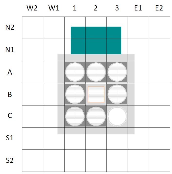
Mini core reactor model with a homogenization grid

Todo

Define the core homogenization grid and associated grid pitches. Since you are using Python, any way of filling the array is allowed. An example of how this can be done is added in comments to the template based input file your created, so start with that if you wish.

Defining the axial homogenization mesh

Now that you have defined a radial overlay mesh, we need to consider the homogenization from an axial perspective. We would like to divide the core into a series of axial regions, each preferably with limited axial heterogeneity. These can also be referred to as axial cuts. Each of these cuts will be given a name, a height. These cuts will eventually result in a 2D (top and bottom reflective) full core heterogeneous Serpent calculation from which nodal cross-sections will be extracted for each radial position in that cut. Eventually, these homogenized axial crosssections will be stacked upon one-another to form the 3D nodal model. To accomplish this, we define the following cards:

parameters.homogenization_axial_mesh = 'SET ME!'
parameters.axial_mesh_bottom = 'SET ME!'

For this model, we would consider that (for all rods out, as would be the typical state for homogenization), there is very little axial heterogeneity over the active height. We therefore suggest using a single axial cut in the active region, with two top and two bottom reflector regions (inner and outer) of 10 cm each. Note that:

• the homogenization_axial_mesh should be specified from top-to-bottom. You can use names such as ('TO', 'TI', 'ACT', 'BI', 'BO').

• The axial_mesh_bottom defines the axial position, relative to the heterogeneous axial core zero point, where the bottom of the axial_homogenization grid should be anchored. This zero point was explicitly chosen when the component models were built, as you assumed some zero point during that phase. In this case, as is typical, the active core centre-line is defined as the axial zero point.

Hint

It is better practice to directly define the mesh bottom as a calculation from known quantities in your script, as opposed to only an answer you found with your own hand calculation – this is more traceable later.

Todo

Define the core axial homogenization grid and associated mesh bottom.

Defining the core state

If you do not specify an explicit core state, the default as defined in the heterogeneous core configuration will be inherited. However, it is good practice to set this explicitly. The call to set this is already in your template, but needs to be completed. As we want to define a hot operational core state, we should use a fuel_temperature of 60°C, moderator temperature of 40°C, and a moderator density from water tables at 1.8 bar.

Todo

Edit the skeleton input for set_state to define the core state in your template to hot operational conditions.

Hint

It is good practice to add an extra argument to set_state of set_state = True/False thereby defining whether the control is inserted in this core model. By default, auto_compose sets all rods at fully extracted.

Visualize your homogenized core model

In the steps leading up to here, you have created a nodal core model. In the next section we will define loadable assemblies to put in this model, but first it is time to see what you have produced. The simplest way to do this, is to perform a visualization of your auto_compose model. You can do this using the command:

>>> oscar5 MINI_CORE.compose.tutorial_operational TUT_CORE visualization

Note here that you have to specify what to visualize, as the script contains both a specification for the core and loadable components. For this reason you use the name you earlier specified for the full-core homogenized model in the command, which will be (TUT_CORE) if you followed the instructions exactly as given in the previous sections.

Todo

Visualize your full core homogenization grid and confirm whether this is the homogenization grid which you intended to produce.

When you visualize your heterogeneous reactor model with the nodal grid overlay, you should see something like the following figure. You can rotate this model and inspect the nodal grid that you have defined.

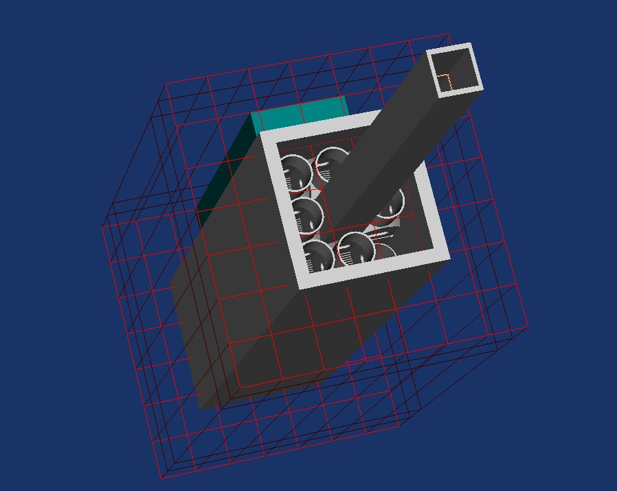
Mini core reactor model with nodal grid overlay

Step 3: Defining Homogenized Models for Loadable Components

Now that we have a core model, it remains to define a homogenized representation for each of the loadable components. In this case we have two of them, namely the fuel component and the control rod follower component.

The fuel assembly

One loadable component input has been automatically added to your template input, and we can use this one for the fuel component. In the case of the fuel model, the input specification is identical to that used in the first tutorial and we will not cover it again in detail.

As a quick recap, recall that we identify the grid_id into which this component is to be loaded, which is 1 in this case for fuel (which is also the default in the script). We can also stay with the setting for 8 burnable layers over the active region.

In this case however, we do not need to specify the additional input for the active lattice cut (burn-up and off-base steps) in this infinite lattice fuel model, as we already did this and ran the calculation for this fuel assembly in the First OSCAR-5 Run tutorial. Here we can use a feature in cOMPoSe which allows you to simply import an existing cross-section set in the so-called HED file format, which is what both the Serpent lattice calculation (post processed by OSCAR-5) and the other OSCAR-5 lattice solver HEADE, produces.

You will note that your template already has an entry for importing an external lattice output (although it is commented out). All you need to do is uncomment this line, and correct the path to the HED file. The relevant HED file has been placed for you at:

../model/lattice/FUEL_LEU—-.HED.

Note that this file only contains cross-sections for the active fuel layer. Although there are five layers defined in this loadable component (defined in homogenization_axial_grid), the auto_compose interface will assume that this mixture data can be used to represent cross-sections for all active fuel layers in this loadable model (in this case the ACT cut). However, using the more advanced features of cOMPoSe, we could have import external files for any of the axial cuts we defined.

Todo

Complete the input for the fuel loadable component and visualize it to confirm that the infinite lattice homogenization model is as you expect. Remember to visualize TUT_FUEL.

The control assembly

Similar to the fuel assembly, we need to create a loadable model for the control assembly. Here we have to adjust some of the parameters, since the control assembly would not share the axial mesh layout of the full core, as was the case for the fuel assembly. Our control assembly has a distinct axial structure which consists of the following regions: a bottom reflector, fuel follower, coupling piece, absorber section and, finally, a top reflector structure. This information was used to construct the heterogeneous model and was further captured in the generation of the auto documentation for the model, which you can open as model_description.html on the top-level of the model this tutorial (Tutorial found here).

We do not need all the heterogeneous detail at this point to construct the homogeneous model of the follower, but at least we should consider which distinct axial zones we would like to define (see figure below). To assist you in this, consider including:

• a 20 cm region below the active core for a reflector zone of the control bottom structure,

• a 59.37 cm active zone for the fuel follower section,

• a 3.85 cm coupling piece,

• a 79.53 cm absorber region,

• and finally a 20 cm top structure region.

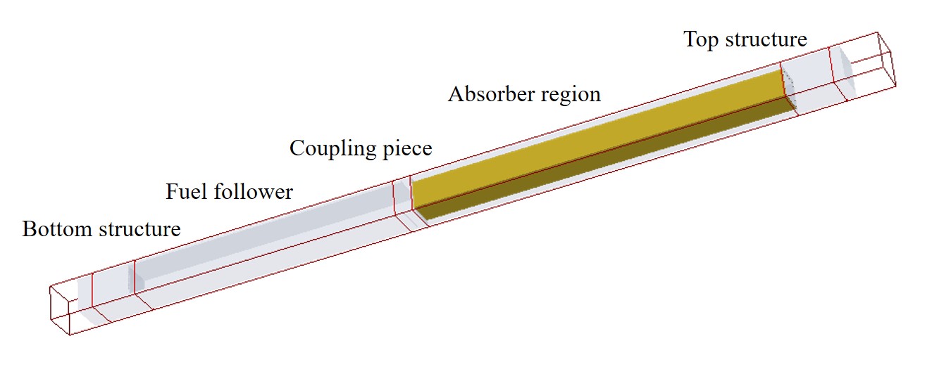
Absorber model with regions identified (structure material greyed out)

Hint

Ensure that you use the same amount of bottom reflector in all your homogenization models (core and loadables), so as to ensure a consistent “all in” seating for all components.

Using this information, you can define an additional loadable section in your auto_compose input for the control rod and follower. To do this, you will have to do the following steps:

1. Copy the full block of input used for the fuel loadable component (starting with create_loadable and ending with build_compose_model).

2. Rename the inf_fuel variable to something else of your choosing in this block. Maybe set it to inf_follower.

3. Update the directory path used to store calculational output for this loadable component. Maybe set it to TUT_CONTROL.

4. Specify a new homogenization_axial_mesh and axial_mesh_bottom for this loadable component. You can copy this from the core model (TUT_CORE) and then adapt it.

5. We have once again pre-calculated the lattice output for the active region of the follower. In this case it was not calculated with Serpent, but with the other lattice code in OSCAR-5 named HEADE. The file can be found at:

   ../model/lattice/CNTRL_FOLLOW.HED.

   Specify this HED file as external lattice mixture to import.

Hint

If you don’t specify a homogenization_axial_mesh and axial_mesh_bottom for a loadable assembly, it inherits the same mesh and zero point as you specified for the core model. Therefore your fuel assembly inherited these parameters from the core model. However the fuel follower model is quite different axially to the fuel and core models and therefore needs these parameters specified.

Todo

Create a loadable input block for the control follower, and visualize it to make sure that you have placed the homogenization mesh correctly.

Step 4: Testing the Nodal Model

Finally we get to the really interesting part of the model building process. In this section we will start exploring our nodal model and estimate the errors associated with using it.

Running full-core cuts to generate cross-sections

Before we can start calculating anything with our nodal model, we must run a series of Serpent calculations to generate cross-sections for all the layers of our core, our fuel loadable component and our control loadable component.

As we are importing the result of existing lattice calculations for the active regions, we would not need to redo these burn-up and off-base calculations in this case, but make sure to revisit the first tutorial to see how this was done if you wanted to regenerate it.

Apart from the single assembly lattice calculations which you will import, all of the standard cut calculations for the core, fuel and control still have to be run though. This will still take a while, and so we have performed these for your already, based on a pre-completed auto_compose input file called operational_core.py in the same directory as where you are now working. This file points to directories in which the results of the relevant Serpent calculations are already present. We will now switch to this file, since all Serpent calculations produced from it are already available in this tutorial.

However, for completeness, if you wanted to recalculate all these cuts, you would need to perform the following commands on your tutorial model to generate all necessary cross-sections. Have a look at these and make sure you understand the process, since it was covered already in the first tutorial. You do not need to perform these steps now.

1. Run all cuts associated with the TUT_CORE full-core model:

   >>> oscar5 MINI_CORE.compose.tutorial_operational TUT_CORE generator --config-file buttercup.cfg --threads 20 --force
   

   Hereafter, the result should be post-processed via:

   >>> oscar5 MINI_CORE.compose.tutorial_operational TUT_CORE update --config-file buttercup.cfg
   

2. Run all cuts associated with the loadable fuel component:

   >>> oscar5 MINI_CORE.compose.tutorial_operational TUT_FUEL generator --config-file buttercup.cfg --threads 20 --force
   

   after which again the results have to be post-processed via:

   >>> oscar5 MINI_CORE.compose.tutorial_operational TUT_FUEL update --config-file buttercup.cfg
   

3. Run all cuts associated with the loadable control component:

   >>> oscar5 MINI_CORE.compose.tutorial_operational TUT_CONTROL generator --config-file buttercup.cfg --threads 20 --force
   

   after which again the results have to be post-processed via:

   >>> oscar5 MINI_CORE.compose.tutorial_operational TUT_CONTROL update --config-file buttercup.cfg
   

After the Serpent calculations are complete, it is good practice to check the Monte Carlo errors associated with these calculations. This is done via the added option given to the post processing of the generator results. For example, to visually check the errors, now for the new operational_core.py input file, for the ACT cut of the full-core (CORE), you could type:

>>> oscar5 MINI_CORE.compose.operational_core CORE ACT generator --config-file buttercup.cfg post --show

This command should yield a map like here, which summarizes the convergence errors for the Monte Carlo calculation.

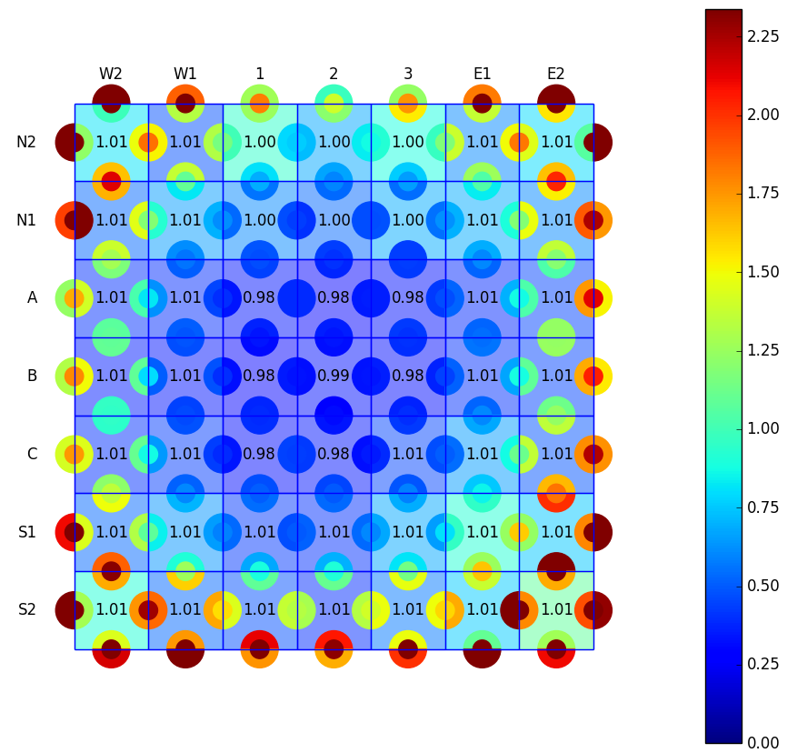
Generator errors in the mini core model

This error map shows a grid of the same size as the nodal overlay grid. Values in the nodes indicate the level of balance achieved in each node. These values should be close to one. Nodes are coloured according to the maximum cross-section relative error in each node. Each segment in the mesh also has two nested circles. The inner circle shows the relative error on the boundary flux estimation. The outer circle is divided into two zones, showing the error on the incoming and out going current respectively.

Todo

Confirm that balance errors, cross-section convergence errors and leakage errors as tabulated from Serpent are within acceptable norms. You would like cross-sections to be converged to within less than 1%, while leakage quantities can be somewhat less converged (maybe a few percent). Balance errors should be less than 1%, but this is sometimes difficult to achieve in such small cores as this is.

Generating equivalent nodal parameters

Up to this point we have not connected our model to a nodal code yet. We want to create a homogenized cross-section library and set up a model for the MGRAC nodal diffusion code. The first step towards this goal is to generate equivalent nodal parameters from our unified model. To achieve this we have to run the library mode for the core and each loadable component.

Since you have covered this process in the first tutorial, it is not re-discussed in any detail here. To do this for all the in cuts in your model, execute first for the core model:

>>> oscar5 MINI_CORE.compose.operational_core CORE library --force

Hint

The command given here runs the library mode for all 2D cuts in the core model. You can instead run each cut separately by including the name of the cut directly after the CORE keyword, for example: … CORE ACT library …

Then for the each loadable component:

>>> oscar5 MINI_CORE.compose.operational_core INF_FUEL library --force

and

>>> oscar5 MINI_CORE.compose.operational_core INF_CONTROL library --force

The --force flag is used to ensure that the POLX calculations will be rerun for all of your models, instead of simply skipping POLX because there are POLX printout files stored from previous calculations.

It sometimes happens that the equivalent nodal diffusion calculation in POLX fails and gives negative flux values. This tends to happen near outer boundaries of large models, where diffusion theory isn’t a good calculational method to use. When this happens, the discontinuity factors are automatically set to 1. It is important to understand if and where this happens in your model. To check where the nodal diffusion calculation failed during the library mode calculations, you can type:

>>> oscar5 MINI_CORE.compose.operational_core CORE ACT library --errormap

This option is only available for active cuts, and you have to specify a cut in the command. This command will show you a core map and failures will be indicated with red lines on the map. If there are no red lines on the grid, then all of the POLX calculations were successful.

Todo

Run the library mode for the core and each loadable component. See if all of the POLX calculations were successful and if the nodal equivalence parameters were properly calculated.

Checking equivalence for the nodal model

We are now ready to build our first nodal model and check equivalence between this and the heterogeneous reference calculations. Equivalence calculations isolate a given layer and allow you to check how well your nodal model preserves important quantities such as reactivity, nodal powers and nodal group fluxes. From equivalence theory we would expect that, in a given layer, you should obtain equivalence if all nodal parameters were correctly calculated. You can perform an equivalence calculation for the ACT layer of the full-core model, via:

>>> oscar5 MINI_CORE.compose.operational_core CORE ACT equivalence --errormap

This step will automatically deploy your nodal model to a 2D MGRAC calculation and perform the nodal solution for the 2D slice in question.

Hint

Equivalence calculations can only be performed for active layers. Reflector cuts cannot be calculated in isolation as they have no source of neutrons.

Todo

Perform equivalence calculations for all the active layers in your model, hence for the full-core, the loadable fuel and the loadable control, to confirm that the generator calculations performed as expected. Note down these results, so that you can later compare this with the replacement case tests in the next section.

The maps produced by this command will show values for the Serpent calculations at the top of each node, followed by that for MGRAC and finally the errors relative to the Serpent results. Maps are generated for power and group-wise flux results.

Checking replacement or reconfiguration errors for the nodal model

One of the most important steps in the construction of the nodal model, is checking the errors associated with introducing your loadable components into the full-core model. This step introduces an error in your nodal model, since the boundary conditions in which the loadable component cross-sections were generated, differ from the real boundary conditions they experience in the full core. This is a necessary evil, as we have to choose typical representative core environments when constructing the loadable models, keeping in mind that they will move around the core and thus change environment from cycle-to-cycle.

In our case both the fuel and control fuel follower models are generated in an infinite lattice environment, which is quite different from what they experience in this mini core model. To check these so-called “replacement” errors, we have to define replacement cases for the active cuts in which we expect these components to be loaded.

We only have three such cases:

1. The full-core active cut with fuel replaced by the loadable fuel cross-sections (INF_FUEL),

2. the full-core active cut with the control replaced by the loadable control model (INF_FUEL), or

3. both replaced with their loadable model counterparts (combined effect, ALL).

The replacement cases are called via the reconfiguration mode in cOMPoSe. To see which reconfigurations the auto_compose interface added for you, you can type:

>>> oscar5 MINI_CORE.compose.operational_core CORE ACT reconf --help

In this case you will see six (as opposed to three) reconfiguration cases available. You should see ALL, INF_FUEL and INF_CONTROL as expected and described in the list above, but also notice that two additional reconfigurations are available, namely INF_FUEL_HED and INF_FOLLOWER_HED. These are added since you specified an external lattice output to be utilized, and thus you can consider these also as legal replacements. The ALL case however, does not include these, and applies only to the primary replacements for each loadable.

We can call the reconfiguration case, for example for the INF_FUEL replacement, via:

>>> oscar5 MINI_CORE.compose.operational_core CORE ACT reconf INF_FUEL execute --errormap

This step will automatically deploy your nodal model with cross-sections for the loadables from a lattice calculation, to a 2D MGRAC calculation and perform the nodal solution for the 2D slice in question.

Please note that although the auto_compose module adds these cases automatically, you can always define more sophisticated reconfigurations yourself. For example, to add a reconfiguration case which, lets say defined as ALL_HED, which replaces fuel and control with their external lattice import mixtures, you could add the following to the end of your script:

rc = parameters['ACT'].add_replacement_case('ALL_HED')
rc.replace(1,inf_fuel.hed_fuel)
rc.replace(2,inf_follower.hed_fuel)

You would immediately notice that a little more understanding of the underlying cOMPoSe system is necessary to accomplish this, but the additional input should also make some reasonable sense to you after analysing it. You will see that this block of code is present at the bottom of your script, but commented out. If you wish to try this option also, just uncomment the block. However, in this tutorial, this kind of interaction between the automated and standard cOMPoSe interface is just demonstrated here, and not fully discussed.

Hint

In cases where reconfiguration errors are too large, possible solutions can be found in more sophisticated coloursets as opposed to pure infinite lattice calculations.

Todo

Check reconfiguration / replacement errors for all loadable components, as well as for the combined effect of all of them. Consider whether these errors are acceptable or not.

Using full core mixtures in your loadable components as advanced option

In some cases it is advisable to use homogeneous cross-section mixtures from the full-core model in building your loadable models. This is particularly true for non-fuel cuts which are sensitive to the radial environment of the component, and would benefit from being calculated in the full-core model as opposed to an infinite lattice arrangement. As an example we can consider the case of the absorber material in the follower-type control rod. If you do not use any advanced options, the cut generated through the absorber axial zone would in actual fact represent an infinite radial absorber, and result in very inaccurate absorber equivalent nodal parameters.

To remedy this, we can choose to rather fetch the absorber cross-sections from a full-core model where the control rod is partially inserted into the active core and is thus surrounded by its typical neighbours.This will notably improve the quality of the absorber cross-sections and discontinuity factors.

The code extract below shows the addition to the loadable follower model to accomplish this:

In this specific extract, we choose to rather take the absorber and coupling piece cross-sections from the full-core model. In particular we choose to select the cross-sections from the full core model in core position B2, for a core state where the control rod is partially inserted to 30%. The auto_compose system will automatically build additional cuts in the full-core (CORE) model, and use them in the nodalisation of the loadable follower component. These cuts are automatically named with the prefix CORE-, and hence we would find an additional full-core cuts named CORE-ABS and CORE-CPL. You could visualize these cuts normally with:

>>> oscar5 MINI_CORE.compose.operational_core CORE CORE-ABS visualization

The excerpt discussed above has already been added to your auto_compose input. This will not affect any of the reconfiguration error checks that you did in previous sections, since these tests were only done for the active regions, thus not the absorber or the coupling piece regions. It will only affect the accuracy of the full-core calculations, which will be done in the next section.

Todo

Perform the equivalence calculation for the CORE-ABS cut and confirm that the nodal cross-sections for the absorber were well calculated.

Summary of 2D cross-section preparation procedure

The procedure described in previous sections has guided us through:

1. Generating cross-sections from 2D cuts through our core and loadable models, with Serpent, using the generator mode.

2. Generating equivalent nodal parameters with these cross-section sets, with POLX , using the library mode.

3. Checking equivalence for the 2D calculations, with MGRAC, using the equivalence mode.

4. Quantifying the errors made when using replacement cross-sections from lattice calculations, with MGRAC, using the reconf mode.

At the end of this procedure you can graphically browse through all of these steps (as opposed to one at a time, as we did in the sub steps), by using the following command:

>>> oscar5 MINI_CORE.compose.operational_core CORE post --show

This is a powerful top-level post processing option that will give you all the information that you need to know how accurate your equivalent nodal parameters are, in 2D models.

Todo

Perform the top-level post processing and browse through the graphical summary for testing your nodal model.

Step 5: Deploy and Test the 3D Nodal Model

Finally, we have reached the point where the final homogeneous model can be deployed and tested in 3D. We can deploy the nodal model to MGRAC and test it by comparing 3D Serpent Monte Carlo and 3D MGRAC nodal diffusion calculations.

We deploy the model using the deploy mode. This is done only on the core model, since it knows about all its constituents and can produce now a single run-time library with all cross-sections needed. You can type:

>>> oscar5 MINI_CORE.compose.operational_core CORE deploy

At this point you have a homogenized cross-section library in the LINX format, ready for use in MGRAC calculations. The very last step in cOMPoSe is to do some 3D tests, in particular, to set up a full-core calculation with both Serpent and MGRAC, with all rods out (ARO), all rods in (ARI) and rods at mid-core (AR50), and compare results.

This step requires that you first calculate the reference Serpent heterogeneous case for these tests, which auto_compose will automatically set up for you. This reference Serpent calculation has been already been run for you and you do not need to repeat it, but the command would be:

>>> oscar5 MINI_CORE.compose.operational_core CORE test ARO reference --config-file buttercup.cfg execute --threads 20 --force

Hereafter we can calculate the nodal solution (simulator) for the same case:

>>> oscar5 MINI_CORE.compose.operational_core CORE test ARO simulator execute --force

Finally, we can test the model by comparing the Serpent and MGRAC calculations:

>>> oscar5 MINI_CORE.compose.operational_core CORE test ARO compare

Todo

Deploy the model and perform the ARO test to confirm that your 2D nodal errors (found with reconfiguration tests) translate reasonably to an overall 3D nodal error. We have already calculated the reference Monte Carlo calculational test for you (for ARO and ARI, so you do not need to repeat this expensive calculation.

Congratulations on completing the nodal modal preparation! You now have a full 3D heterogeneous model (from Part 1 of this tutorial) and a full 3D homogenised nodal model for the mini core. You also have a knowledge of how accurate your nodal model. The only thing remaining to do, is use your model in a calculational application.

Step 6: Run an application with your nodal model

Now that the model has been deployed and tested, we can run a calculation with it. At the end of Part 1 of this tutorial, you created an application input in OSCAR-5 to calculate the bank worth of the control rods. An important inherent feature of OSCAR-5 is that applications can be seamlessly deployed to any code package connected to it. Let us work in the application input file that we created for you, which can be found at: ../projects/base.py. This input performs a ARO and ARI calculation, and calculates the total bank worth from these.

We will now perform the same calculations, but with the nodal model you just developed. You will have to do two things to accomplish this:

1. Set the desired nodal configuration you want to use - in this case you only have one. To do this you will have to add the line to your input script for the application:

   model.nodal_representation = assemblies.nodal_configurations.CO()
   

2. Secondly, you will have to tell OSCAR-5 that you intend to run the calculation with MGRAC. To do this, we add the argument --target-mode MGRAC to the execution command for the calculation.

Hint

By default, the first two letters of the name of your cOMPoSe full-core model name (which in this case was CORE) is used to reference your nodal configuration. Since you may have many nodal configurations associated with your reactor, you need to tell a given application which one to use.

You can then run the rod worth calculation using the command:

>>> oscar5 MINI_CORE.projects.base --target-mode MGRAC execute --force

and view the results by typing:

>>> oscar5 MINI_CORE.projects.base --target-mode MGRAC post --force

to post process the result. We can compare the rod worth calculated here with the results that you have obtained in Part 1 and relate the differences to the expected error margins defined when we developed the nodal model.

Todo

Perform the bank worth calculation with the nodal model, and compare your answers to those obtained in Part 1 of this tutorial. Do they compare as expected?