The First OSCAR-5 Run tutorial tutorial gave you
an overview of the system and the modelling capabilities
in OSCAR-5 (stands for the Overall System for the CAlculation of Reactors, generation
5). This tutorial will focus in greater detail on how to build a reactor model in OSCAR-5 and
then the next tutorial (Full Core Applications) will pick up where this one ends and use a reactor
model to do some real life applications such as core-follow calculations.
In Part 1 of this tutorial you learned how to build a
heterogeneous reactor model. You learned about:
Building an assembly library with geometry, material and state specifications for all reactor components.
Defining a reactor configuration, state and loading.
Performing a rod worth calculation in Serpent, using the full core heterogeneous reactor model.
Now in Part 2 of this tutorial, you will learn how to create a homogeneous nodal model from
the heterogeneous one and deploy this homogeneous model to the OSCAR-5 nodal solver called
MGRAC (stands for the Multi-Group Reactor Analysis Code). Since this homogenization process
involves making various approximations, it is important to keep track of the errors introduced
in the model. You will also learn how to to quantify the MGRAC model accuracy
compared to the detailed heterogeneous Serpent model.
This tutorial ends with the same application example as in Part 1, that is a rod worth calculation,
done with the homogeneous model in OSCAR-5.
Attention
After this tutorial, you will be able to…
Define a nodal mesh over the heterogeneous reactor model in OSCAR-5.
Generate few-group homogenized nodal equivalence parameters, from full-core 2D core calculations
and from infinite fuel lattice calculations.
Deploy a homogeneous nodal model to the nodal diffusion solver MGRAC.
Quantify the accuracy of the nodal model compared to the full-core reference heterogeneous model.
Perform a rod worth calculation using the full core homogeneous nodal model.
Your facility is investigating different reactor design ideas. A mini core has been defined for
this study. You have been given specification documents and have been tasked with creating
the calculational model for this reactor design. This design is unique and therefore you have
no previous models to start with, you will have to build the components and core configuration
from scratch. Since this is a conceptual study, you can suffice with simplified assembly models,
thereby not getting lost in the detail at such an early stage of the study.
You decide to create both a Serpent model and a nodal model of the reactor. You will test the
accuracy of your nodal model by quantifying the errors introduced at each stage of construction,
ending with an expected accuracy for your final 3D full-core nodal model as compared to the
reference heterogeneous 3D full-core Serpent model. Finally you will do a rod worth calculation
with both models, to confirm whether your nodal results have the accuracy that you predicted.
Recall from the First OSCAR-5 Run tutorial that the main entry point to the OSCAR-5 system
is the construction of a unified, code-independent system model. This was done in Part 1,
the Mini Core Heterogeneous Model tutorial. Once this model is built, the user can generate a
code-specific geometry and material input from this model, and code-specific application input,
allowing the use of this model in reactor calculations.
The unified code-independent heterogeneous model can be used directly in codes such as Serpent
and MCNP (stands for Monte Carlo N-Particle Transport Code), as these codes can handle the
detailed model geometry. Therefore code-specific input generation for these codes is mostly
automated in OSCAR-5. However a nodal diffusion solver such as MGRAC requires a model
to be divided into large blocks or nodes in which all detail is approximated by a homogeneous
representation. Additional model preparation is required when generating code specific input
for a nodal solver. cOMPoSe (stands for the OSCAR Model Preparation System) is used to
systematically move from the heterogeneous unified description (using point-wise cross-section
data) to a set of homogenized mixtures with energy condensed to a few-group representation.
There are many factors to take into account during this homogenization procedure and the
final outcome is a model with a limited number of large (typically assembly pitch sized) meshes,
which would allow a very fast calculation of the neutron flux distribution. We want the nodal
model to capture as much of the neutronic behaviour of the heterogeneous model as possible.
The basic approach in building a nodal model has been discussed in First OSCAR-5 Run tutorial.
Please make sure that the basic concepts discussed there are understood before we move
on to this more realistic case. The calculational procedure in the cOMPoSe system typically
involves the following steps:
The first step is to select a full-core configuration that fits the best the intended purpose of
the homogenized model. Since the cOMPoSe system attempts to retain as many properties
as possible from the detailed model, the bulk of the homogenization process is performed
on the full reactor scope, as opposed to single assembly models.
For this selected core configuration, a coarse radial overlay mesh is chosen, which define
the node sizes radially. This is typically done in such a way that the fuel pitch is preserved,
so that fuelled assemblies fill one node. Ex-core region meshing is more flexible, but it is
good practice to keep nodal meshes more or less cubic.
Note
Often the ex-core structures does not align with the fuel assemblies or even have the
same pitch. This is not a concern, as the nodal grid does not have to align with the core
or ex-core assemblies. cOMPoSe will homogenise the materials within a node using flux-volume
weighting, regardless of their composition.
Next, a number of axial slices are chosen along the height of the model, with each slice
capturing important features of the model, while attempting to limit the amount of axial
heterogeneity within a slice, since detail within a slice will be homogenized axially. This
effectively divides the model into a number of two-dimensional layers (radially spanning
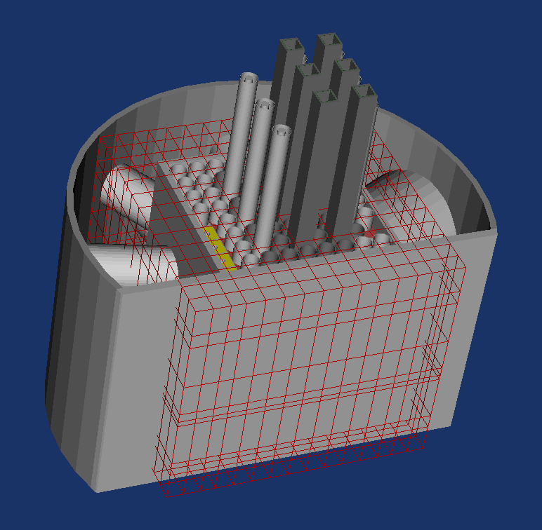
the full reactor model). As a practical example, the image below shows such a nodal mesh
overlay for the SAFARI-1 reactor model.
Example of a nodal mesh overlay for a heterogeneous model.
Homogenized cross-sections are then calculated on the nodal mesh for each axial layer, by
performing a two-dimensional transport calculation over the entire slice, using Serpent.
Generalized Equivalence Theory (GET) is used to ensure that reaction rates and leakages
are preserved for each node. The major advantage of this approach of using full-core slices
is that complicated static features, such as the ex-core facilities encountered in research
reactors, can be treated explicitly and accurately.
Fuelled assemblies, or any other assemblies that either undergo state changes (e.g. burnup),
or do not stay in a fixed position in the core, need additional treatment. This is because
for a fast operational support tool, we do not want to re-homogenise the entire core every
time the fuel configuration or state changes. Thus, fuelled and other loadable assemblies
are treated in a more traditional fashion, by performing assembly-level lattice / coloursets
calculations in approximate environments. These calculations also account for burn-up
and state changes. Currently these lattice calculations can be done with the lattice physics
code HEADE (HEterogeneous Assembly DEpletion), or with Serpent. Since the lattice
environment is an approximation to the core environment, this step can be a major source
of error, and its effect must be carefully monitored when creating a homogeneous reactor
model. This error monitoring is an important feature that is automated in cOMPoSe.
cOMPoSe will then stack all two-dimensional layers together to form a three-dimensional
model. Since axial leakage is not preserved in generalized equivalence theory (the transport
calculation is done for 2D), this is another potential source of error. The nodal representation
for each loadable component is also stored. How and when these components
are loaded, is determined by the specific application or calculation you choose to perform
at a later stage.
A few of the steps described above can introduce errors into the nodal model, which is discussed
below. During each step of this homogenization process, the system gives feedback on
the errors incurred (as compared to the detailed heterogeneous model). This is done by deploying
the homogeneous model to MGRAC, performing a nodal calculation and comparing the
results to the same model with heterogeneous full detail (as calculated with Serpent).
This feedback includes cross-section generation errors, equivalence errors, and loadable component
replacement errors.
Cross-section generation errors are associated with the level of Monte Carlo convergence
attained during calculation of the 2D cuts and (if using Serpent) the loadable component
lattice calculations.
Equivalence errors typically indicate how well equivalence parameters (cross-sections,
discontinuity factors and form factors) can compensate for the move from transport to diffusion
theory, and from the heterogeneous to the few-group homogeneous representation.
If the process is fully successful for all nodes (some numerical issues can occur such as in
reflector nodes far away from the core), there should be near-exact equivalence in terms
of reactivity and nodal powers/fluxes.
Replacement errors are introduced when adding loadable components homogenized from
approximate environments into the full core model.
Finally the full three-dimensional error, which includes axial leakage errors, as well as
other axial effects such as homogenization and the movement of control rods. There are
no axial discontinuity factors as it is expected that diffusion theory can handle the (usually
homogeneous) axial solution adequately, which is generally the case.
Hint
Since cOMPoSe provides a detailed feedback on the errors incurred in the homogenization
process, you can identify which approximations lead to large errors and you can refine your nodal
model to within acceptable and well quantified error margins.
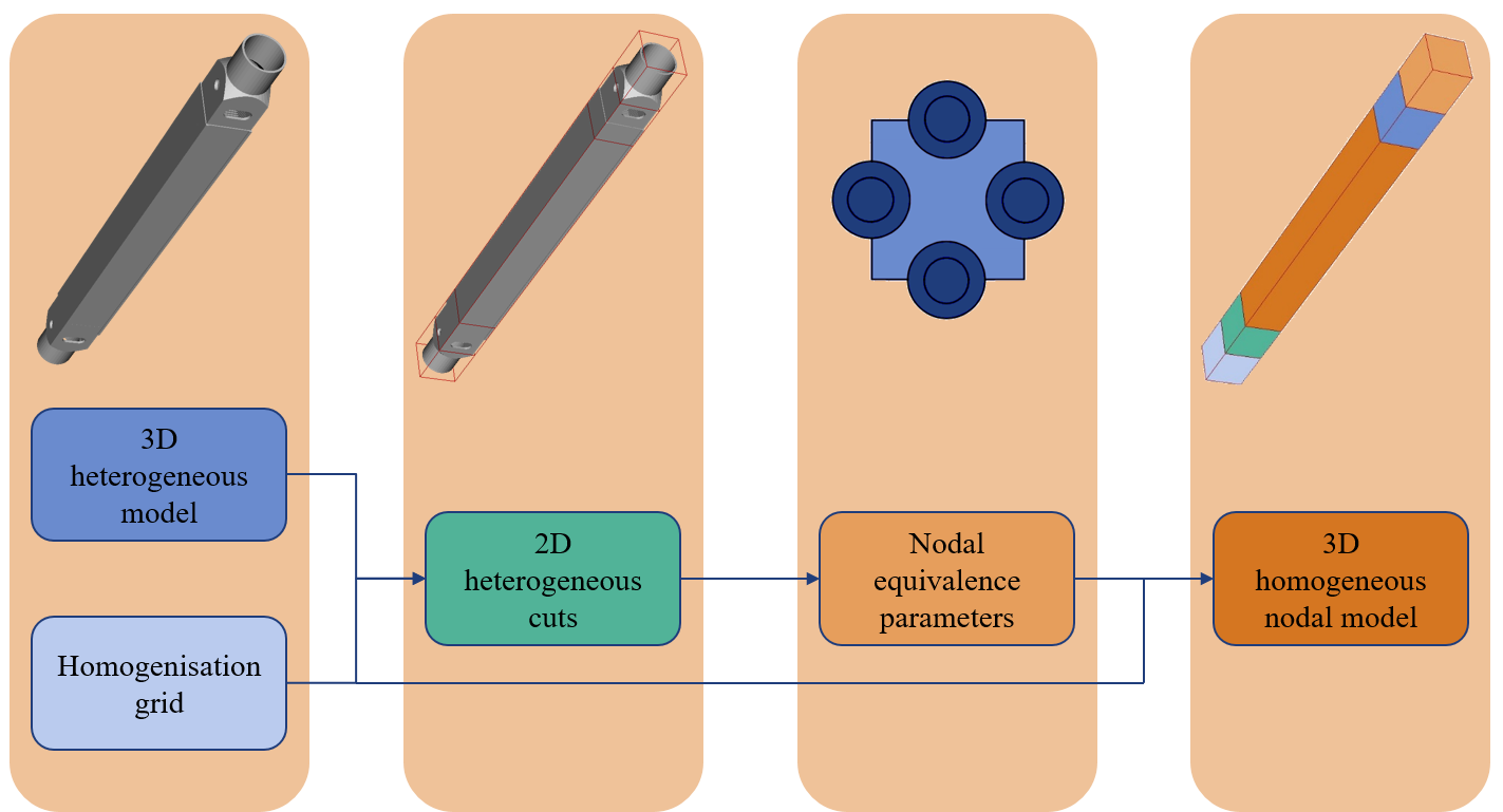
In summary, the cOMPoSe procedure is given in the figure below. This diagram shows the steps
involved in going from the unified model to a nodal modal. Note that the procedure shown here
is done once for the core, and once for each type of loadable component (such as fuel type 1,
fuel type 2, burnable rig, etc.). Therefore you should end with a set of nodal models. Only when you
use the final nodal model (i.e. setup code-specific input for the nodal diffusion solver MGRAC)
will the loadable nodal models be “loaded” into the core model and a homogeneous nodal core
model be created, as defined by the set of nodal models.
Schematic of the cOMPoSe procedure, for a loadable fuel assembly
In this tutorial Serpent is used to generate cross-sections for the two-dimensional slices. Lattice
calculations (for the loadable components) have been performed by HEADE for a number of
discreet state conditions of the assembly and cross-sections are generated for each point in the
assembly state space. These calculations have been pre run for you and we will simply import
the results into our model.
After generating the cross-sections, the POLX code is used to represent these cross-sections as
a function of state-parameters (such as burnup, fuel temperature, moderator density, etc.). POLX
also performs the equivalent diffusion calculations which are an integral part of equivalence
theory to generate the discontinuity factors – this is done in POLX so that the capability is
available for any connected transport solver. The set of few-group equivalent nodal parameters
for each material include node-averaged cross-sections, discontinuity factors at the assembly
boundaries and flux/power form functions to allow the reconstruction of heterogeneous detail
during the full-core global diffusion calculation.
Finally, the LINX code combines all homogenized equivalent nodal parameters from the twodimensional
slices (core and lattice models), into a single run-time cross-section library. This,
together with the nodal mesh, forms the final homogenized three-dimensional model, suitable
for use in the nodal diffusion solver MGRAC, to be applied over multiple operational reactor
cycles. The codes HEADE, POLX, LINX and MGRAC are all part of the OSCAR-5 nodal code
package.
In MGRAC, the calculation of the steady-state neutron flux distribution is based on the solution
of the three-dimensional multi-group diffusion equation by means of a modern transverseintegration
nodal method for Cartesian geometry (steady state and transient capability exists
in MGRAC). The specific nodal method applied is known as the Multi-group Analytic Nodal
Method (MANM).
This tutorial covers the cOMPoSe calculational procedure in detail, and results produced from
the nodal model are compared to the reference Serpent solution via the interface provided in
OSCAR-5. However no further discussion is given on the individual codes involved and the
user is referred to the set of user guides for the nodal code itself, and its associated tutorials, for
further insight into these codes. Earlier versions of these codes also formed part of the OSCAR-4
code package. In OSCAR-5 they are still present (although updated) and are used internally on
your behalf to generate and use your nodal model.
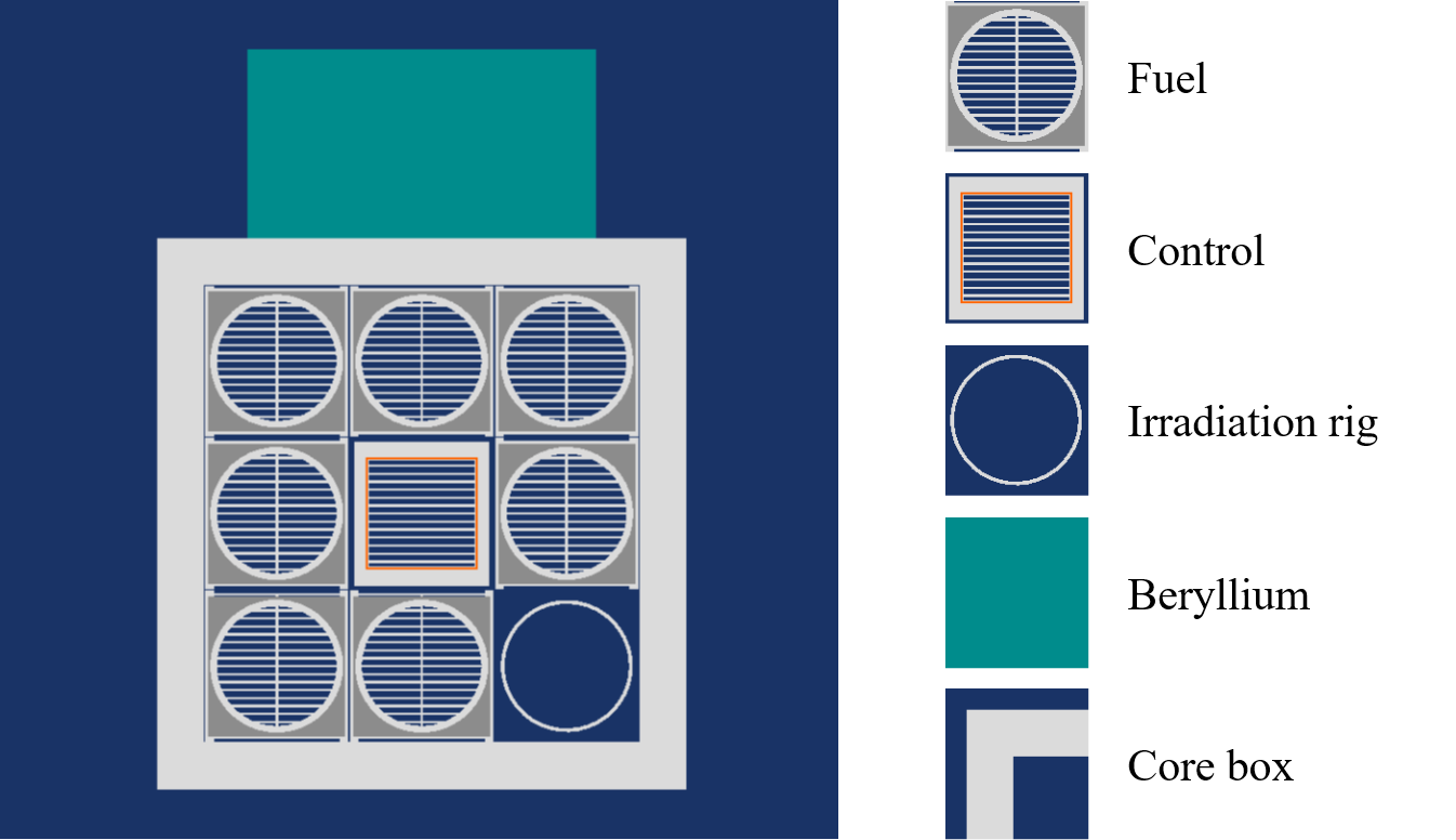
The mini core design as specified in Part 1 is repeated here
in the following figure. The model is a 3x3 core with seven plate-type MTR fuel assemblies surrounding
a central absorber (fuel-follower-type control assembly). There is also an in-core irradiation
facility in one corner. This core is moderated by light water and the only other reflector material
is a large ex-core beryllium block next to one side of the core. In this tutorial you will generate,
test and apply the three-dimensional homogeneous nodal model for this mini core.