Step-by-Step

In this chapter you will create a working reload and core-follow set for a newly built SAFARI-1 reactor full core model. There are many ways in which you can approach such a task but we will demonstrate our suggested way using the OSCAR-5 system. You will be referred to appropriate sections in the OSCAR-5 user guide for information on other methods and tools.

Getting Started: The OSCAR-5 Setup for this Scenario

In order to proceed with this tutorial, OSCAR-5 should be installed on your system. The project space for this tutorial can be found at

<TutorialPath>/SAFARI_1.

Please note that <TutorialPath> is the path to your OSCAR-5 Tutorial Series and is typically (but does not have to be) set to ~/oscar5_tutorials/, where ~ refers to your home directory. This model can also be found on GitLab.

The actual calculational codes within the OSCAR-5 system should of course be pre-installed and their paths defined within the OSCAR-5 configuration files.

The commands shown in the steps below are often illustrative and do not have to be run again. This will be indicated where appropriate. Unless you are working in PyCharm, make sure that the virtual environment is activated in the terminal you are working, by typing

>>> conda activate oscar5

Hint

In the step-by-step that comes, you do not have to execute all commands (you can of course), but at typically only perform that defined as a “Todo”.

For this tutorial, we will use the SAFARI-1 benchmark to perform all the necessary calculations. The model description for the SAFARI-1 model that you will use can be found here:

<TutorialPath>/SAFARI_1/document_browser.html

Todo

The first task for you in this tutorial, is to browse the auto generated model documentation produced for the SAFARI-1 model (using the html link given above). Have a look at the fuel design, control rod design, core layout and also the nodalisation used to produced the homogenized model.

Step 1: Studying the Existing Reactor Model

Given that you are familiar with the building of reactor models after completing the tutorial Building a Reactor Model with OSCAR-5 Part 1 and Part 2, we will only have a quick look at the existing model of the SAFARI-1 reactor, which will form the basis of this tutorial. The model is based on the SAFARI-1 benchmark specification, and also contains its own full set of OSCAR-5 generated model description documentation.

Assembly models

One notable difference between the assembly models that you have encountered in previous tutorials and those in this model, is that many of these have parts, or even the full assembly model, imported from an existing MCNP input. One example of only parts being imported is the fuel assembly, found in

<TutorialPath>/SAFARI_1/model/leu_fuel_assembly.py.

In this case the fuel plate bundle is constructed with the PlateAssembly macro, while all the other regions, such as the end adapters, are imported from MCNP. We will have a quick look at a simpler case where the whole model is imported from MCNP. If you open the file

<TutorialPath>/SAFARI_1/model/hollow_beryllium.py,

you will see the following import statement:

from core import *
from material_library.moderators import LightWater
import materials
from extensions.mcnp_model_importer import *

Notice the reference to extensions.mcnp_model_importer, which gives access to the built-in system interface with MCNP input. Inside the build() method, you will see the familiar material definitions, followed by the following statements:

src = create_mcnp_importer(utilities.path_relative_to(__file__, 'sources RRT_SAFARI-1_Model_v2.i'))
# pick a universe
u = src.universe(20)
u.materials = {120: lwt, 112: al, 130: be}
# extract all cells from the universe
cells = u.extract_cells()
# add all the cells to the components
hb.add_cells(*cells)

You can see that it starts by specifying the path to the MCNP input that should be used, whereafter it indicates the specific universe and materials that correspond to this assembly, and finally adds the cells that were extracted from that universe to this model.

You are welcome to look at the other assembly models and compare their contents to what you now know about modelling of assemblies in OSCAR-5.

Todo

Visualize some of the assemblies, especially those that were not used in previous models, such as the shielded ringas or the pool.

The core configuration and facility loading

The basic structure of the core configuration is the same as before, although it now contains more loadable facilities, a number of stationary reflector assemblies, and several control rods that are grouped into different banks. To see what the reactor you will be using to do full core calculations on, visualize the file

<TutorialPath>/SAFARI_1/configurations/base_hot_core.py.

It is possible to have several different configurations that can form the basis for different types of applications. Examples of this can be found in the set of reactor models included in the OSCAR-5 distribution.

The facility loading is an interesting case, given that it forms part of the bridge between the high level conceptual model of the assemblies and core configuration, and the physical core for which calculations are performed. Take a look at the file

<TutorialPath>/SAFARI_1/facility_loading/tutorial_C1109_1.py.

It should look quite familiar, except that the core map now contains assemblies that were not imported with the fresh importer as before. Where the data comes from and how to obtain it is discussed later in this tutorial.

The cOMPoSe model

This is the first model you encounter that was not built with auto_compose interface. It is quite an extensive model, and creating it is beyond the scope of this tutorial series. To see the axial cuts, visualize the model with the command:

>>> oscar5 SAFARI_1.compose.operational visualization

In this cOMPoSe model, both the fuel and control follower sections are taken from infinite lattice environments.

Step 2: Obtaining a Starting Inventory

We will be working with SAFARI-1 cycle C1109-1 as our starting point. In order to initiate an inventory at that point, it is assumed that you have an OSCAR-4 inventory. This means that you already have a database of partially burnt assemblies, and thus you are of course not starting with a fresh core.

OSCAR-5 offers many options for obtaining a starting inventory. Although we plan to use an OSCAR-4 model as source in this tutorial, the same process is used if you have data defined in some other format. OSCAR-5 uses the concept of an importer, which provides the set of rules for reading the historic data files. Although a series of typical importers are predefined for you, you can easily add your own. In this case though, we will use an importer called the OSCAR4HistoryImporter.

OSCAR-4 keeps track of material compositions of all loadable components. For each loadable component, e.g. fuel assemblies and follower type control rods, there are associated component history files. The history file contains the irradiation history of the particular component. It lists date and time stamped material data including fuel exposures and nuclide number densities at specific time points. In this specific historic OSCAR-4 model, data was written to the history at two time points for each cycle i.e. at the Beginning-of-cycle (BOC) and at the End-of-Cycle (EOC). These history files then make up the starting inventory for the new model that you intent to use. In this step you will import elements from this already existing inventory so that it becomes the starting material composition data for partially burnt components. Note that we intend to import all assemblies that were already burned at the beginning of cycle C1109-1, as fresh assemblies will be added in facility loading actions (next section). Of course we have no guarantee that the historical model has the same meshing or list of isotopes as our new model, but this should not be a problem as the importer will take care of these differences.

Residual isotope treatment

Before we get into the step-by-step process, we have to introduce additional information on the process of creating an OSCAR-5 element inventory. We want it to be code independent. However, it is typical for deterministic reactor modelling tools to keep track only of a subset of the most important actinides and fission products. This is the case for the historic OSCAR-4 inventory which we are importing from. This list typically contains between 20 and 50 isotopes, and allows the core solver to perform core depletion with this subset of neutronically important isotopes explicitly during the core diffusion calculation. The remainder of the fission products and actinides (called residual isotopes), not selected for explicit core tracking (typically a few hundred of them) are often modelled as a single macroscopic lump material. This material is not depleted explicitly at the core diffusion stage, but simply tabulated during the lattice code calculation as a function of burn-up. To capture their effect during the core calculation, a lookup from the lattice code output for the lump macroscopic cross-section is performed when needed.

We face a challenge then, since our aim of defining a code independent inventory, would require that our database carry explicit number densities for all fission products, actinides and structural material. How do we reconstruct these when importing?

The OSCAR-5 approach to this is the following:

Perform, for each loadable, burnable assembly type, a so-called exposure calculation, which depletes the assembly in an infinite-lattice (or your own choice of colourset) environment at nominal conditions. At each burn-up step, all microscopic isotopes present in the assembly are tabulated as a function of burn-up. This database is stored for later use. Just a note, that OSCAR-5 contains two ways to do this – either via a dedicated exposure calculation (which we will show you below) or via a special input option added to the lattice calculation input when performing lattice cut calculations with Serpent.

Import the historic assembly data, and instruct OSCAR-5 to fetch information on the residual isotopes from the exposure database by matching the exposure of the imported assembly to that of the exposure database. In that way we replace the macroscopic lump with an explicit list of isotopes. You could even choose a single representative isotope if you prefer, as OSCAR-5 allows you to choose an isotope and calculate its number density in such a way as to retain the reaction rate of the lumped material. B-10 (boron 10) is a typical choice for such a representation.

We are not going to cover the exposure calculation in detail here, as the process is very similar to that which you did in the first tutorial to perform a lattice cut calculation for a fuel element. However, to see what the input looks like, you can open the file:

<TutorialPath>/SAFARI_1/exposure/leu_fuel_assembly.py

To run the exposure calculation, we would use the following command:

>>> oscar5 SAFARI_1.exposure.leu_fuel_assembly --config-file buttercup.cfg execute --threads 20

after which you can post process the result to produce the database with

>>> oscar5 SAFARI_1.exposure.leu_fuel_assembly --config-file buttercup.cfg post

You do not need to perform this calculation, as the exposure database for both the fuel and control follower components has already been created, and you will just use it.

Importing historic assembly data

As we would like to perform calculations starting from cycle C1109-1, our starting inventory should have data up to the end-of-cyle C1108-1. We start of by inspecting the inventory importing script. This is a complete script and you will not have to change it, but simply understand its contents. Open the file:

<TutorialPath>/SAFARI_1/facility_loading/tutorial_initiate_inventory.py

to inspect the script. The script has been divided into two sections as shown below. As has been the case in previous tutorials, the top part of the script imports some relevant modules from OSCAR-5 and sets some preliminaries. We note that the facility management modules are imported, as well as the specific history importer we intend to use, along with the core configuration and assembly library which you have seen before in most of the previous scripts. You will note that the path to the inventory is set, as well as the path to the facility loading database. The former defines the space where the inventory files will be stored, and the latter refers to the file which will keep a list of facility loading states.

import os
from applications.facility_management import *
from core import *
from extensions.oscar_history_importers import OSCAR4HistoryImporter, residual_isotope_options
from ..configurations.base_hot_core import model
from ..model import assemblies
model.inventory_manager.inventory = utilities.path_relative_to(__file__, '../SAFARI_1_inventory_tutorial')
model.facility_manager = utilities.path_relative_to(__file__, '../SAFARI_1_facility_tutorial')
parameters.model = model

Next we set important run parameters for preforming the initialization of the inventory and the facility database.

# Time at which inventory should be populated
parameters.time = '2011-10-10 00:37:20'
# ===============================================
# Import fuel elements
source_path = '/home/oscar/projects/oscar5_tutorials/FULL_CORE_APPLICATIONS/historical_model'
importer = OSCAR4HistoryImporter()

# specify base file paths
importer.base_path = {
    'CNTRL_': os.path.join(source_path, 'assdef', 'CNTRL_ROD.BASE'),
    'F_LEU-': os.path.join(source_path, 'assdef', 'FUEL_LEU.BASE'),
}
# library file
importer.library = os.path.join(source_path, 'library/SAFARI_LIBRARY.LNX')

# history
importer.inventory_path = os.path.join(source_path, 'hist')
importer.residual_isotope_treatment = residual_isotope_options.replace_with_exposure
importer.load_time = '2011-10-10 00:00:00' # Slightly earlier to allow decay from previous cycle

# -------------------------------------------------
# Fuel assemblies
fuel = parameters.add_batch(assemblies.SAFARI_1_LEU_fuel, importer=importer)
fuel.add_all(importer.inventory_path, 'EF*L.HIST')
# -------------------------------------------------
# Control assemblies
followers = parameters.add_batch(assemblies.SAFARI_1_LEU_fuel_follower, importer=importer)
followers.add_all(importer.inventory_path, 'C*L.HIST')
if __name__ == '__main__':
    main()

We begin by setting parameter.time, which is the date at which a planned facility change should take place. Typically this would be the date and time when the core was physically loaded. However, in this case it will also be interpreted as the time at which the inventory is to be populated.

Next we define the setup for the importer which will search the source (set here via the source_path variable) and fetch burn-up data. In this case we define the importer as an OSCAR4HistoryImporter. In the OSCAR-4 world (as is the case for the OSCAR-5 nodal solver), each assembly (defined by its HIST file) has a type, and the basic properties of each assembly type is defined in a so-called BASE file. We therefore define the base_path and the path to the old nodal cross-section library to tell the importer about the types of assemblies in the historical model (we supply the type name and the file name here). From these historical BASE files (and the old cross-section library), the importer knows information such as the axial material mesh of the old assemblies and the list of microscopic isotopes that were historically tracked. You can learn more about the file types associated with the nodal solver in the OSCAR-4 user-guides and tutorials if you wish, but it is not necessary for this process at this time.

Three more pieces of information is passed to the importer:

The inventory_path is defined relative to the top-level source path. This is the directory which will be searched for assembly data.

We set residual_isotope_treatment to replace_with_exposure. This makes sure that the inventory is not only populated with the limited list of microscopic isotopes tracked in the historical model (typically between 20 – 50 in nodal codes). The more complete list of fission products and actinides (maybe 300 – 400) may now be populated in the code independent inventory based on the burn-up value of the given layer in the assembly. The additional isotopes are interpolated (via burn-up) based on a predefined database of isotopes tabulated from a single assembly infinite lattice burn-up calculation for each assembly type. This database is created via a so-called exposure calculation which OSCAR-5 performs on an assembly type. As discussed above, we accept that this database already exists and you will use it.

We set the importer.load_time. This is the time at which the historical data source is queried for assembly isotopic and burn-up data. This time is typically set to some time before the parameter.time (facility loading time), but after the EOC of the previous cycle when data was saved to the historical model. In practice then, the old inventory is searched for a time stamp that is earlier than or equal to the load_time. If such as step is found, the assembly is added to the inventory at its historically saved time-step (and not at the load_time). Note that imported data is always added to the inventory at a time-stamp found in the historical database, as this is the time stamp for which the data is valid.

Finally, we create assemblies via defining batches of certain types. These new types now have to match some of the heterogeneous assembly types we defined in the OSCAR-5 model directory and which thereafter reside in the assembly library. We go further and assign a filter to to each batch to assist the importer in selecting which elements have to be imported in that batch. In this tutorial we import a fuel and a control batch.

To execute the script, import inventory, and update the facility loading database, we run:

>>> oscar5 SAFARI_1.facility_loading.tutorial_initiate_inventory execute --force

Todo

Perform the initialization of your inventory and facility loading database. You can thereafter browse the inventory folder and see what files have been added to it.

We might be done at this point, but we anticipate that we would like to later have a second independent core-follow calculational line with Serpent. To that end, we would need a second inventory for future use, as each each core tracking code should store its own depletion information.

Todo

Repeat the above task, but create a second inventory called SAFARI_1_inventory_tutorial_serpent in anticipation of later having a second independent core-follow line with Serpent. You will have to change the name of the target inventory in the script.

Step 3: Facility Loading

Now that we have a starting point in time, we can perform the actual facility loading for cycle C1109-1. This script is relatively simply, and serves to store the loading of the core facility at the load time of the cycle. It performs two functions:

Add assemblies to the inventory which are fresh in this cycle, by the same batch mechanism as before.

Create a loading of type actual and define the core load map for this cycle. The actual keyword implies that this is an action in reality, as opposed to generating a loading for, lets say, some conceptual core. The loading will be stored at time parameter.time, which will be the time stamp used to retrieve this loading in the future.

The facility loading input is primarily just an administrative support tool to makes sure that the states of the facilities are updated. Here again we provide you with a completed input. Open the file:

<TutorialPath>/SAFARI_1/facility_loading/tutorial_C1109.py.

The content of the file should now be rather self-explanatory. Browse the file and make sure the content is clear to you. To execute the script, import inventory, and update the facility loading database, we run

>>> oscar5 SAFARI_1.facility_loading.tutorial_C1109_1 execute --force

Todo

Create a core loading and save the loading in the facility loading database. Note that the file SAFARI_1_facility_tutorial.py is created and contains the loading for this core.

Step 4: Performing a Reload Calculation

It is now time to perform an analysis of the proposed core. The required parameters to define a core as acceptable is highly variable. It differs between reactor types, but even between similar reactor designs simply because of the way that the safety analysis for that reactor was defined. It is therefore important for a modelling support system to allow a high level of customization in defining the set of reload parameters and how to calculate them. In OSCAR-5, we go about this in four stages outlined below. Remember that in OSCAR-5 a result may be calculated with any code connected to it – hence any of the calculated reload parameters discussed here may be equally calculated by the nodal solver or a Monte Carlo code – however, some choices would be more practical than others. For the sake of this part of the tutorial, we are going to perform the calculations with the nodal solver. To define a reload calculation, and generate a report on the results:

Define the set of predictive_lines you require. A predictive line has a given core loading determined by placement of fuel, control, irradiation rigs and samples, and a cycle progression spanning BOC to EOC. You may have a number of these. For example, you may a have line from which you want to extract power peaking related quantities, and as such want to define an allowable core state which maximizes peaking. In the case of SAFARI-1, this could imply a hot core state, where all power producing rigs are unloaded, as to maximize the power density in fuel elements. From such a calculation you could aim to extract quantities such as maximum relative peaking factor, maximum local heat-flux or maximum power density. Similarly, you could define a reactivity limiting core from which you could aim to extract quantities such as shutdown margin, control rod worth or excess reactivity. You could also add a line from where you would like to extract utilization information such as typical fuel burn-up or isotope production yields, and load the most typical isotopic load into the target positions.

Define a set of results or trending parameters to extract from the predictive lines. These give an overview of how the cycle would progress and typically would include time-dependent plots of bank position or mass change over the cycle. This could also include maps of powers, fluxes or masses at various points throughout the cycle.

Next we define specific results to calculate. Here we think of power peaking, bank worth or other derived quantities. OSCAR-5 has a series of these known to it, and you can select from an available list, or even add your own. OSCAR-5 will assess the list of results requested, and set up a set of calculations, called cases, to generate the results.

Finally, you choose which of the above you would like to include in the final report, and provide some additional information such as titles, limits or specific formatting. The requested parameters are then collated into both a pdf and html report.

In the coming sub-sections, a series of code-snippets are extracted from the relevant input files. Note that in some cases, the order of code extracts do not follow exactly the order of the input files, and might be grouped differently to facilitate the explanation.

Perform the predictive line calculations

To get you started, we have prepared an input file for you that already contains sufficient definition to produce a simplified reload report. Actually, we have prepared two input files. The reason for this is that a large part of the input required to generate a reload report, is common to all cycles for which you would want to do this. Hence it makes sense to separate the cycle-independent part of the input into a reusable definition of what you required in a given reload report, and have a second input file, specific to each particular cycle. In this case you will find the following two relevant files:

reload/generic_report.py - this is the common input to all cycles for a given definition of what should be included in a reload report.

reload/tutorial_C1109_1.py - this is the cycle specific input used to perform the calculations and generate the report for cycle C1109-1.

Lets start by having a look at the reload/generic_report.py file. As before, we are going to highlight some important parts of the input file, and select relevant parts to reproduce in the blocks below as needed. We look at the part of the file defining the predictive lines:

from ..configurations.base_hot_core import model, assemblies
parameters.model = model
peaking = parameters.add_predictive_calculation('peaking',
                                                'Predictive calculation for the peaking limiting core',
                                                steps=[0.1 * units.days,
                                                       0.25 * units.days,
                                                       0.75 * units.days,
                                                       1.5 * units.days,
                                                       3.0 * units.days])
peaking.bank_search = ['control', 'regulating']
peaking.bank_search.target_keff = 1.00

Here we fetch our standard model for the core as built in the configuration stage, and create a prediction line – we call it peaking. The standard model, as defined in:

../configurations/base_hot_core.py

does not have fuelled target plates loaded in irradiation positions, and is thus already the correct core layout for use in a peaking calculation. We add the predictive line called peaking, and define its cycle progression. The specification for the day increments is followed as specified, with the last step automatically applied multiple times until the planned cycle length is reached. The fine scale steps at the start of the cycle is added for accurate modelling of Xenon build-up. Planned cycle length however is only specified in the cycle specific input, as cycles may vary in planned length. Finally we choose which banks to include in the bank searches, as the cycle progression will perform critical searches and thus automatically find the critical bank at each step in the cycle. We also set for this purpose the target k-eff to define the model specific value for criticality (models generally have an off-set in their critical prediction).

We can also have a look at the definition of a second predictive line called reactivity. The relevant parts of the input for the second prediction line are given below:

# Rig loading (Dummy rigs) c3 = assemblies.SAFARI_1_Homogenized_Mo99(name='Mo99C3')
e3 = assemblies.SAFARI_1_Homogenized_Mo99(name='Mo99E3')
g3 = assemblies.SAFARI_1_Homogenized_Mo99(name='Mo99G3')
b6 = assemblies.SAFARI_1_Homogenized_Mo99(name='Mo99B6')
b8 = assemblies.SAFARI_1_Homogenized_Mo99(name='Mo99B8')
d8 = assemblies.SAFARI_1_Homogenized_Mo99(name='Mo99D8')
f8 = assemblies.SAFARI_1_Homogenized_Mo99(name='Mo99F8')
f6 = assemblies.SAFARI_1_Homogenized_IPR(name='IPRRF6')
d6 = assemblies.SAFARI_1_Homogenized_IPR(name='IPRRD6')
rig_map = \
    [[0,   1,  2,  3,  4,  5,  6,  7,  8,  9],
    ['A',  _,  _,  _,  _,  _,  _,  _,  _,  _],
    ['B',  _,  _,  _,  _,  _, b6,  _, b8,  _],
    ['C',  _,  _, c3,  _,  _,  _,  _,  _,  _],
    ['D',  _,  _,  _,  _,  _, d6,  _, d8,  _],
    ['E',  _,  _, e3,  _,  _,  _,  _,  _,  _],
    ['F',  _,  _,  _,  _,  _, f6,  _, f8,  _],
    ['G',  _,  _, g3,  _,  _,  _,  _,  _,  _],
    ['H',  _,  _,  _,  _,  _,  _,  _,  _,  _]]
reactivity limiting reactivity =
parameters.add_predictive_calculation('reactivity',
                                      'Predictive calculation for the reactivity limiting core',
                                      steps=[0.1 * units.days,
                                             0.25 * units.days,
                                             0.75 * units.days,
                                             1.5 * units.days,
                                             3.0 * units.days])
reactivity.model.add_assembly_facility_load_map('Irradiation-position', rig_map)

In this case all fuelled rigs are defined, placed in a rig map, and loaded into rig positions. You have already learned how to do this in the Mini Core tutorial, so refer back if this rig loading seems unfamiliar. These fuelled rigs are loaded as we would like to have the model in its most reactive state for the sake of conservatism. For now ignore the rest of this input file, and lets move on to the cycle specific input so that we can run these predictive lines. The cycle specific input can be found in reload/tutorial_C1109_1.py and contains only a few simple definitions:

from generic_report import parameters, reactivity, peaking

parameters.start_time = '10/10/2011 00:37:20'
parameters.cycle_name = 'C1109-1'
parameters.working_directory = utilities.path_relative_to(__file__, 'tutorial_C1109_1')
parameters.planned_cycle_length = 30 * units.days

This file should be largely self-explanatory by now. The parameters.start_time is important, as this is the time at which a facility loading will be fetched from the facility loading database. We also note the import of the generic_report module, and the setting of some basic parameters and the cycle length for this cycle.

To now perform the two predictive line calculations, we can either launch them both at the same time via:

>>> oscar5 SAFARI_1.reload.tutorial_C1109-1 prediction --target-mode MGRAC execute --force
>>> oscar5 SAFARI_1.reload.tutorial_C1109-1 prediction --target-mode MGRAC post --force

or call, for example, only the peaking line via:

>>> oscar5 SAFARI_1.reload.tutorial_C1109-1 prediction peaking --target-mode MGRAC execute --force

Todo

Run both peaking and reactivity predictive lines which simulate the cycle progression for the core with and without targets loaded in irradiation positions.

Extracting cycle trend parameters

As discussed in the introduction to the core reload analysis, we next define which parameters we would like to extract directly from the prediction lines to characterise the cycle progression. In this case we choose (from the generic report file):

days = parameters.extract(cycle_progression, reactivity)
banks = parameters.extract(bank_positions(bank='control'), reactivity)
masses = parameters.extract(u235_mass, reactivity)
boc_map = parameters.extract(u235_mass_map(at=BOC), reactivity)
eoc_map = parameters.extract(u235_mass_map(at=EOC), reactivity)

You will see here that we identify the result of interest with a keyword, followed by the predictive line from which we would like to extract it. In this case we ask for cycle_progression, bank_positions, u235_mass and u235_mass_map at BOC and EOC. For a full list of possible keywords, consult the user manual. In this case, we choose them explicitly from the reactivity calculation, as we want these parameters extracted from the core with targets loaded. To extract these parameters, we have to post-process the prediction calculations. We do this, simultaneously for all prediction lines, via:

>>> oscar5 SAFARI_1.reload.tutorial_C1109-1 prediction --target-mode MGRAC post --force

The post processing step here is optional, as the overall post-processing can be called at the very end, and subsequent steps which need post-processed results will call the post-processing automatically. You thus do not need to perform any task at this step.

Define specific results to calculate

The next step is to define the set of particular results of interest to calculate. Here we have freedom to use the power of the scripting environment in order to define particular results and manipulate them to report correctly defined safety and utilization parameters. The input file you have contains quite a number of examples - and we show a few in the input file extract below. These parameters require additional calculation, as they often require tallies or additional solution options to be activated at the time-points of interest. From the input file we have:

avg = parameters.calculate(average_power_density, peaking, 0)
mx = parameters.calculate(maximum_power_density, peaking, 0)
hottest_channel = parameters.calculate(maximum_power_density_channel,peaking, 0)

total = configure_banks(all=['control', 'regulating'])
all_in = parameters.calculate(total.banks_inserted(), reactivity, 0) # keff with rods in
all_out = parameters.calculate(total.banks_extracted(), reactivity, 0) # keff with rods out

This block shows how some specific results, such as k-eff, average power density or maximum power density with given bank position can be calculated. Once again, for each requested result, you specify from which line to take it, and at which time-point during the cycle. These results to be calculated are grouped together by the code into a set of calculational scenarios, or cases, which you can launch in a batch, or of course as usual one at a time. To spawn the calculation for these requested parameters, use the command:

>>> oscar5 SAFARI_1.reload.tutorial_C1109-1 cases --target-mode MGRAC execute --force

after which you should again post-process the results via:

>>> oscar5 SAFARI_1.reload.tutorial_C1109-1 cases --target-mode MGRAC post --force

Todo

Calculate all requested parameters and results for all cases. You once again do not need to perform the post-processing step here.

Define the reportable quantities

Not everything you calculate has to be reported, and the reported value is often a derived quantity as compared to what was calculated. To facilitate this, the next step is to collate all the above into a set of reportable results. The following input file extract shows a series of such definitions of quantities to report.

parameters.report(days, 'Days')
parameters.report(banks, 'Bank Positions')
parameters.report(masses, 'Core U235 Mass')
parameters.report(boc_map, 'BOC U235 Mass Distribution')
parameters.report(eoc_map, 'EOC U235 Mass Distribution')

parameters.report(mx / avg, 'Peaking Factor', ranges=(None, 3.5), fmt='{:.2f}'.format)
parameters.report(mx, 'Peak Power Density', fmt=format_unit(units.W / units.cc, '{:.2f} W/cc'.format))
parameters.report(hottest_channel, 'Peak Power Channel')

The above extract only shows a few of the results identified for reporting, but you should be able to get a sense of how these are handled. Each reportable result is given in terms of the previous extracted and calculated parameters, is flagged with a name, and some further customization such as setting limits and defining formatting is optional. The system will know when a given quantity is a 1D-plot, a map or simply a single-valued result, and report it appropriately.

The reporting process is highly customizable. In essence the process up to now has defined a series of available quantities for reporting. Once these are defined, you process and calculate the final reportable quantities with a post-processing step. This is done via:

>>> oscar5 SAFARI_1.reload.tutorial_C1109-1 --target-mode MGRAC post --force

Todo

Post-process the report results in preparation of the report compilation.

Building the report

We need to provide the report builder with a template of how the results should be put together in the report itself. This is done by building a report template, which uses a lightly marked up text based description called restructured text (or rst files). For the set of reportable results you have defined, we have already built a basic report template for you, which you can browse under reload/report_template/. Here you will see a simple top level index file called index.rst which refers to two chapters – the first called summary and the second called cycle_description (these reside in the associated rst files also). You can have a look at both the summary.rst and cycle_description.rst files in order to see how the reportable result names you defined in the previous step are placed in the report. Of course the use of restructured text format will take a little getting used to, but remember that you generally only

You will note that you input script refers to this report template toward the end of the script with the line:

You can therefore have multiple templates for multiple types of reports and use them as required. We are now ready to produce our report. This requires two steps:

Prepare the report

Generate the final version of your rst based report with the actual data as opposed to the named result place-holders currently in the template via:

>>> oscar5 SAFARI_1.reload.tutorial_C1109-1 --target-mode MGRAC prepare-report

After this step, you will see that a populated version of the rst files has now appeared within your working directory (should be reload/tutorial_C1109_1/report/source).

Build the report

To compile and build the actual final report in both pdf and html formats, use the command:

>>> oscar5 SAFARI_1.reload.tutorial_C1109-1 --target-mode MGRAC build-report

This step will produce a browsable html report under reload/tutorial_C1109_1/report/build/html/index.html and a pdf version under reload/tutorial_C1109_1/report/build/latex/C1109-1.pdf.

Todo

Prepare and build the final report in both html and pdf formats. Browse the report and consider the behaviour of the proposed core.

Step 5: Performing a Core-Follow Calculation

We assume that time has now passed and the cycle has operated (in reality) and reached EOC. It is now our job to perform the core-follow calculation, which will update the isotopics of the assemblies in the core to their EOC state. In order to perform the depletion calculation, we first process the plant data, and then perform the simulation.

Processing plant data

The first step in a core-follow calculation is to process the reactor operational data or plant data. OSCAR-5 has a built-in plant data processor. For this part of the tutorial, which is GUI-based, you can follow along with the instructions as we go, and you do not have to wait for a task description to move on. To start the process, execute the following script, which is a generic script placed automatically inside any reactor space you create:

>>> oscar5 SAFARI_1.core_follow.process_plant_data

The application window should open as in the following figure.

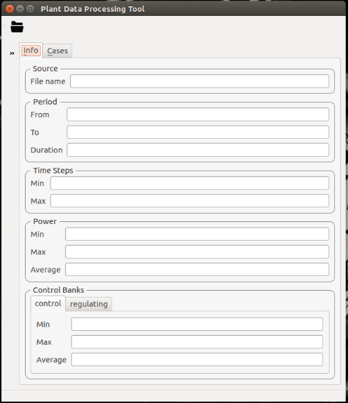
../_images/input_pannel.PNG — Plant data processing application window

Click on the file icon in the top left-hand corner, which will enable you to select the plant data for processing. For this tutorial, we have already placed the plant data dump file from the reactor in the benchmark space. To access the aforementioned data, navigate to the plant_data folder, and select the 1109-1Adroit.csv file. Click on the maximize icon to reveal the plant data plot, as seen in the following figure. The plot indicates the reactor power and control rod bank positions as a function of time.

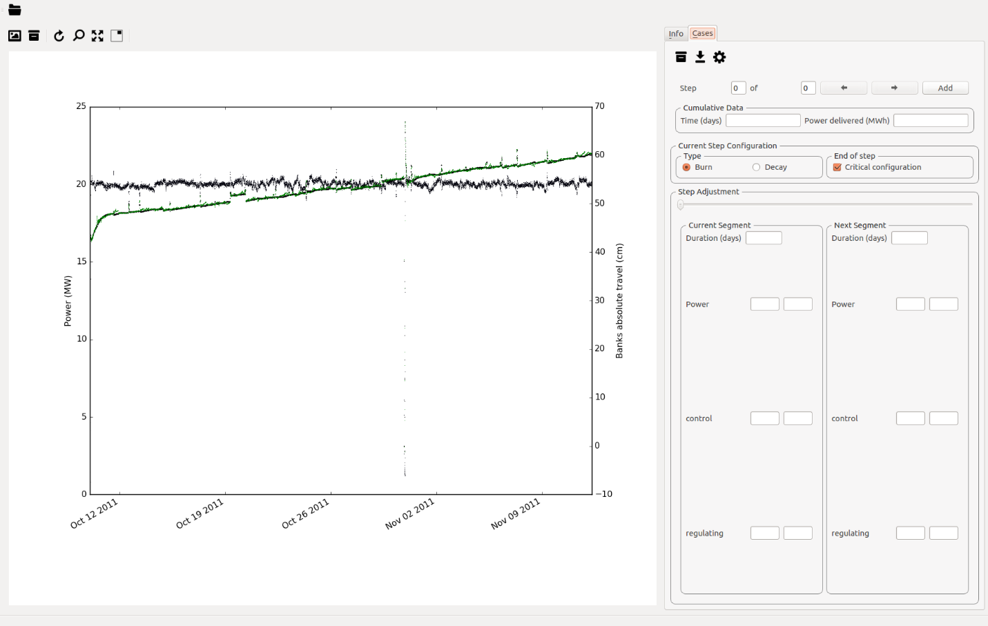
../_images/loaded_csv.PNG — Loaded plant data

The next step is to add critical steps, and burn steps on the graphical representation of the plant data. This is done by selecting the “cases” tab. In the options panel and select add. This will add a burn step on the plant data. The user can now select the characteristics of the step, and define it as a critical burn step, non-critical burn step or a decay step. This choice will depend on the operational characteristics of the reactor, at the specified time step. The duration of the time step can also be varied between very small time steps and a maximum time step (customizable, but here set to 3 days), depending on how rapidly the plant data is changing. It is recommended that at the Beginning of Cycle (BOC), the user specifies a few extra small non-critical time steps to account for rapid changes related to control rod movement and Xenon behaviour. For your convenience we have prepared a plant data file with burn steps for the first couple of days of the cycle. To open the burn step file, select the download icon in the top left corner of the options panel, navigate to the core follow folder under your OSCAR-5 tutorial set, and select the C1109_1_tutorial.pkl file.

If the aforementioned is completed successfully, the burn-up steps will appear on the plant data graph as seen in the following figure. You will see that a few burn steps at the BOC have been added to the plant data, it is now your task to add the rest of the critical burn-up steps.

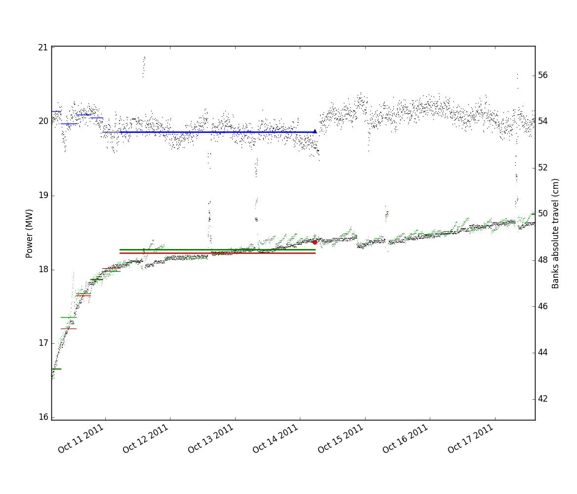
../_images/image-1.png — Plant data with burn steps at the Beginning of Cycle (BOC) – zoomed view

A plant data processing file with burn steps for the entire cycle C1109_1 was added to the core follow folder. When proceeding with the core-follow calculations use the C1109_1_final.pkl file.

Running a core-follow calculation

As with many of the other scripts in the system, the manager utility allows the automatic addition of a core-follow cycle input to the system. You can then populate the script yourself thereafter. For example, if you wanted to add a cycle named TUT_C1109_1 to an existing OSCAR-5 model, you would:

>>> oscar5 SAFARI_1.manager core-follow TUT_C1109_1 --start-time '10/10/2011 00:37:20' --configuration base_hot_core

Note here that we have pre-specified the configuration and the cycle start time.

Todo

Generate a templated core-follow input with the command above. Browse the file to see which data you will have to set to complete the input.

You now have to customize this input. Set the following parameters in the input file:

Set the inventory manager to SAFARI_1_inventory_tutorial. This points the core-follow calculation to the inventory of fuel assemblies which you created earlier.

Set the facility manager to SAFARI_1_inventory_tutorial. This database contains the loading of the core at the given start time, as added by you earlier.

Set the nodal configuration to assemblies.nodal_configuration.Op(). This specifies which nodal representation to use when deploying this model to the nodal code, in this case to the standard operational model created for the SAFARI-1 benchmark.

Set the plant data to ../plant_data/C1109_1/1109-1Adroit.csv. This refers to the plant data file received from the reactor, which you processed to produce the step wise representation.

Set the irradiation history to C1109_1_final.pkl. This file is the result of the plant data processing you performed in the previous step, but in this case does not refer to your produced version, but to a reference file we produced earlier to ensure consistency with the remainder of the tutorial.

Once you have defined these few parameters, it is time to run the core-follow calculation. You can do this via:

>>> oscar5 SAFARI_1.core_follow.TUT_C1109_1 --target-mode MGRAC execute -- force

Following the calculation, you can inspect the result via

>>> oscar5 SAFARI_1.core_follow.TUT_C1109_1 --target-mode MGRAC post --show

Run the core-follow calculation for cycle C1109-1 with the nodal solver, and analyse the behaviour of the critical estimates throughout the cycle. If you wish you can use the pre-completed input named tutorial_C1109_1.py. Also look through the working directory structure under core_follow and find the output file from the nodal solver MGRAC. Open it to see what kind of results are produced by the nodal solver itself.

Step 6: Creating an Independent Core-Follow Line

Now that you have a working core-follow set for your nodal model, it is good practice to validate this set against a high fidelity code such as Serpent. We will now set up an independent core-follow line in Serpent and repeat the core-follow calculation. All the work in this regard has however already been done. You simply have to update the inventory to which the calculation is pointing (as you earlier defined a separate inventory for the high-fidelity line) and point the core-follow script to Serpent. You can do this via:

>>> oscar5 SAFARI_1.core_follow.TUT_C1109_1 --target-mode SERPENT --config-file buttercup.cfg execute --threads 20 --force

Once again, since this takes a while, the result of this core-follow calculation has already been post processed and saved for you. In order to compare the results with the nodal solver, you can open the result of the Serpent run via (this now points to the one which we ran for you):

>>> oscar5 SAFARI_1.core_follow.tutorial_C1109_1 --target-mode SERPENT post --show

This should open the same graphical display as before, but this time show you the results form Serpent. You should also note a small icon top left of the window, which allows you to compare your result to other cycle data. You can navigate through this option to select the output of the MGRAC post processing, namely TUT_C1109_1/MGRAC/C1109_1.res. You should now be able to compare the runs.

Todo

Post process the Serpent core-follow calculation, and compare the results to those you obtained with the nodal solver. Are these differences within expectation? What would be your expectation and how would you check in OSCAR-5 what differences you can expect for this comparison (hint: think of the cOMPoSe process).