Introduction

Congratulations on completing the previous two in-depth tutorials that gave an overview of the OSCAR-5 system (your First OSCAR-5 Run tutorial) and model building (Building a Reactor Model with OSCAR-5 Part 1 and Part 2) side of the system. This current tutorial will focus on some key applications of the OSCAR-5 system, i.e. core-follow and reload calculations. Additionally, related activities such as importing an inventory, loading a facility, and sharing number densities between codes will also be covered.
Background
In this tutorial we focus on some calculational applications for real world reactor problems. As part of your OSCAR-5 distribution you will note that a series of full reactor benchmark problems are included. These serve many purposes, such as support to verification and validation of OSCAR-5, training of users as well as demonstration of the typical usage of more advanced features in the code. These benchmarks also provide you with a good starting point for modelling your own reactor, as many different designs are covered in these test problems. There is a specific user guide covering these problems which you will see later. However, in this tutorial, we will move away from the tutorial space you have been using up to now, and perform the steps described here on the SAFARI-1 validation problem included in the OSCAR-5 benchmark set. This reactor and experimental description originates from a published International Atomic Energy Agency (IAEA) database for research reactor code validation (which is also the case with the other benchmarks distributed with OSCAR-5).
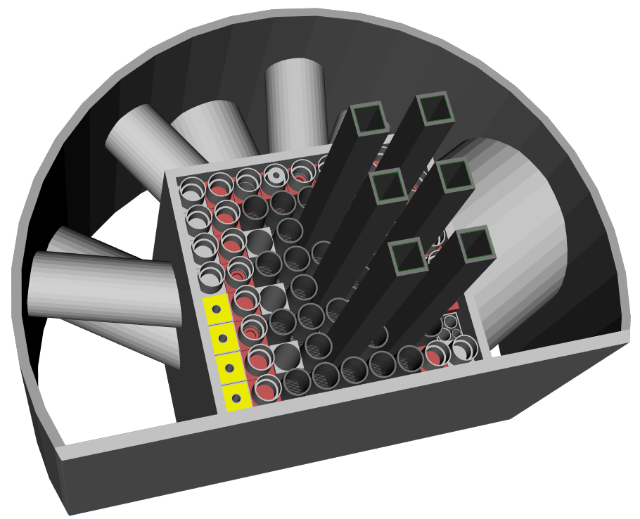
OSCAR-5 model of the SAFARI-1 benchmark
The objective of any reactor analyst is to simulate the reactor, but this is a process rather than a single step due to the varied nature of reactor operations and the data required at different points of the operating process. The interrelated and cyclic nature of the feedback between operation and calculation is illustrated in figure below.
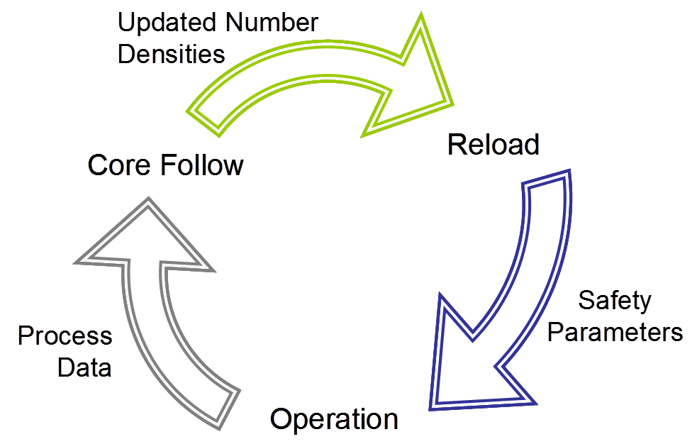
A typical reactor calculational cycle
After the completion of a reactor cycle, plant data is available for use in a simulation to update the burn-up and number densities of the assemblies used in that cycle, with the process data obtained from the plant computer. Thus, before doing a reload for one cycle, one must perform a core follow calculation of the previous cycle.
It is of the utmost importance to be able to track the number densities of several active nuclides, especially fissile material and decay products. This is the primary purpose of performing core follow calculations, and it is important to use the most accurate and up to date process data from the plant for the purpose of inventory tracking.
In this tutorial we assume that you want to start following this process with your new OSCAR-5 model. However, to get into the process, we first have to find a starting point.
You will learn how to get a starting inventory for your newly built model, load a facility with a set of assemblies from your inventory and then do some reload design calculations for the given core. Assuming that the cycle actually occurred in reality, we move on to perform the core-follow calculation for the cycle after its completion. There will be no detailed discussion on the model building process for the SAFARI-1 benchmark, but you will be given the opportunity to browse the model as part of this tutorial.
Attention
- After this tutorial, you will be able to…
Import an inventory from an historical OSCAR-4 model to your new OSCAR-5 model, and load a facility for the coming cycle.
Perform a series of reload calculations to confirm that safety and utilization requirements for the proposed core are met
Process plant data, and then set up and run a core-follow calculation with your nodal model for the cycle.
Deploy the core-follow calculation to Serpent to obtain an independent high fidelity core-follow solution.
The Scenario
You are in the process of migrating your reactor simulation tools from OSCAR-4 to OSCAR-5. You have a functioning OSCAR-4 core-follow set and you have just created a full-core nodal model with OSCAR-5. Now you want to create a starting condition for your new OSCAR-5 models, and model your first reactor cycle in OSCAR-5.
You will need a starting fuel inventory for your model (to be taken from your OSCAR-4 model as example in this case) as well as a planned core loading for the coming cycle. Finally, you would need plant data from the reactor once the new cycle has finished its operation to model fuel depletion in the core. After performing the reload analysis and subsequent core-follow calculation for the cycle, confirm the accuracy of the nodal model by running an independent core-follow calculation in Serpent for the same cycle.
The OSCAR Approach
To perform this work, we will go through four steps, each with its own input file and application in OSCAR-5. We will:
Create a script dedicated to import an existing inventory into the OSCAR-5 inventory manager. There are many ways in which this could be done, and the scripting environment makes it easy to customize this for whatever format you have the data defined in (text files, spreadsheets or other code packages). Typically this data contains, for each fuel assembly in your storage pool or core, a description of the axial distribution of burnup (and potentially radial) and isotopic number-densities. In this case, we will assume that you are migrating from an existing nodal code, namely OSCAR-4. In OSCAR-4, inventory information for each fuel element was stored in a so-called history file, which contains the required information in time-stamped format. After defining the data source, and choosing the time-point for import, you will specify which fuel elements to import. Finally, the script is executed and the OSCAR-5 code-independent inventory is populated. If you have defined a nodal model for your core, specific inventory files for the nodal code will also be created.
Next the facility loading has to be performed, which places a subset of assemblies into a chosen configuration – normally for your core, but it could of course serve to load elements into other facilities such as the pool, the vault or other storage racks. For this task, you will define a cycle specific script, complete it and execute the script. You can also create different types of loadings, such as actual (as it happened in the core), or design (as you are planning it) to name but two.
Now that the core is loaded, we can perform some analysis on the proposed loading, in order to confirm that the safety and utilization parameters meet their respective requirements. OSCAR-5 houses a flexible interface for defining your own custom set of reload parameters which you would like to check against their respective limits. These parameters can then be calculated with all codes connected to OSCAR-5, and an automated report is produced summarizing what was defined. The customizable aspect is quite important, given that different reactors have slightly different definitions of the same parameters. Prime examples hereof would be parameters such as shutdown margin, excess reactivity, peaking factors and predicted cycle length. To perform the reload calculation, we again develop a script, and execute it to perform the reload analysis.
It might be of interest to be aware of a second approach to producing a reload report. As an alternative, we could consider using some of the code specific features included in some of the OSCAR-5 sub-codes. For example, the nodal solver in OSCAR-5 contains an automation assistant called OASYS, which has the capability to produce a reload analysis and report specific to the nodal solver. OSCAR-5 also supports this OASYS sub-code, and can auto-generate the necessary input to run any of the various options available in OASYS. We will not spend much time on this approach further in this tutorial, but this feature is valuable to know for users who used OASYS as part of the OSCAR-4 code system, and would like to continue doing so. To perform reload analysis in this way, we would deploy the OSCAR-5 model to OASYS and then continue to work in that environment.
Next we march ahead in time and reach the end-of-cycle. At this point plant data for the past cycle is available from the reactor, and we can proceed to perform a core-follow calculation. Here we have to think of two distinct steps. The first is to analyse the plant data (power levels, control rod positions, temperatures and energy delivered as a function of time). It is typical to have a look at the granularity of the data (in this case it will be quite fine – order of minutes) and then to process the data into a reasonable quantization, to allow for an accurate simulation of the cycle, while still retaining acceptable calculational efficiency. This typically means to divide the data into two kinds of steps –
fluxsteps to calculate the reactivity and neutron flux distribution in the reactor at a given time point, andburn-upsteps (spanning typically hours to days of real time), which performs the depletion of reactor materials with the last available fluxes. Your task will be to use the tools available in OSCAR-5 to process the plant data, and the second task will be to create and run a script to simulate the cycle. As before, you can deploy this core-follow application to either the nodal solver MGRAC or the Monte Carlo solver Serpent.
Symbols and Abbreviations
BOC Beginning-of-Cycle
cOMPoSe OSCAR Model Preparation System
EOC End-of-Cycle
GUI Graphical User Interface
IAEA International Atomic Energy Agency
MCNP Monte Carlo N-Particle Transport Code
OSCAR-5 Overall System for the CAlculation of Reactors, generation 5
SAFARI-1 South African Fundamental Atomic Research Installation, unit 1