Step-by-Step

We now proceed in a stepwise manner, view the already completed inputs which have been set up for this scenario, and execute them.

Getting Started: The OSCAR-5 Setup for this Scenario

In order to proceed with this tutorial, OSCAR-5 should be installed on your system (see installation manual). Furthermore, the tutorial documents, we will work through in this tutorial series, use examples and semi-completed inputs from a number of different reactors to illustrate various aspects of the code system. The specific input files used in this first introductory tutorial may be found on GitLab.

Within this structure you will find various sub-directories, which represent the typical OSCAR-5 workflow. The actual calculational codes within the OSCAR-5 system should of course be pre-installed and their paths defined within the OSCAR-5 configuration files. We suggest that you use PyCharm as an editor in this tutorial set, as it provides a helpful environment for developing and running Python scripts, but you are of course free to use any editor of your choice. If you choose another editor, note that it might not be as “Python-aware”, and you might have to set the general Python environment for OSCAR-5 manually. This is achieved by entering the following command in the terminal in which you are working:

>>> conda activate oscar5

Keep in mind that since OSCAR-5 employs an in-house developed Python-based reactor analysis platform (called Rapyds), a large amount of the class structure and available source code is accessible to the user and you can dig into the system to whatever depth you wish. However, this tutorial will not address this aspect.

Hint

In the step-by-step that comes, you do not have to execute all commands (you can of course), but at typically only perform that defined as a “Todo”.

Step 1: Building the Heterogeneous OSCAR-5 Fuel Assembly Model – the Materials and Geometry

So the first step is to develop a 3D representation of a single fuel assembly, with regards to geometry and material layout. This is done by accessing the constructive solid geometry module in OSCAR-5 and defining the set of required materials, cells and surfaces. Let us begin with defining the materials.

Note

In OSCAR-5 we generally centralise all required materials in a materials.py file inside the model directory.

To view the current material definitions, open the following file in your editor (simply click on it in the PyCharm project tree view):

<TutorialPath>/SINGLE_MTR_ASSEMBLY/model/materials.py

Here <TutorialPath> is a path to your OSCAR-5 Tutorial Series – and is typically set to ~/oscar5_tutorials/, where ~ refers to your home folder.

Inspect this file, and browse through the OSCAR-5 user manual and select the section on building a material library material library.

You will notice that each material is actually defined by a small routine, which defines a mixture of isotopes. More details on developing your own materials will be covered in a Tutorial 2. For now, note which materials are available in this example.

Next we inspect the geometry of the 3D representation of the fuel assembly. The intent now is not to fully understand all input (this comes in the the next Tutorial), but to introduce the approach and basic constructs involved.

Open the file <TutorialPath>/SINGLE_MTR_ASSEMBLY/model/fuel_assembly.py. In this file, you will notice three sections:

The top of the file contains a comment block, which gives some context to the modelled component. Note that the comments are demarcated via triple quotation marks.

Next we have the import section of the file. Here we select which Python packages in the OSCAR-5 system we need to use in order to build the fuel model. You will notice here packages like fuel_assembly, which contains fuel assembly construction tools, the units package which allows you to work directly with units of your choice and the materials package which you browsed earlier.

Moving a little further down, we discover the build() routine. This routine constructs (and returns) the fuel assembly model and is what we will be concerned with primarily in this tutorial. This routine defines what are the important parameters in constructing plate type fuel assembly.

In the first part of the build routine, a plate-type fuel macro (named PlateAssembly in this case) is used to generate a typical plate-type fuel element in the active region. You will notice that a number of typical design parameters for the plate-type fuel is set in this section.

After the basic construction of the active region of the fuel element, a few dedicated geometric regions are added to the model to allow for a simple representation of the top and bottom adapter structures of the assembly. We will model these in much more detail in the next tutorial, but for now this is sufficient.

If you look in more detail in the macro and cell construction, you will note that each physical region (fuel plates, top adapter and bottom adapter) have all space outside of them filled with water (all the way to infinity). This is in tune with the typical combinatorial geometry approach in many reactor physics codes of having components that fill all space, which then get clipped when they are inserted in the core lattice later on. For simple regions, where the outside space is easily definable, feel free to do this. Alternatively, see the next point.

Towards the end of the build routine, you will notice a few further constructs, such as the complete_universe function, which fills all remaining cells with water. This feature is quite useful in cases when the geometry is somewhat complicated and constructing water cells to fill the remainder of the space is a non-trivial task.

You will also see a call to a routine named construct_bundle. A bundle in OSCAR-5 is a collection of primitives which are flagged as burnable. As you used a PlateAssembly macro, the system knows which parts of the assembly are supposed to be burnable (but you can override this), and thus allows the contents of these cells to be controlled by the burnable material manager.

Finally, the __main__ routine at the end of the file is called when you run this script; we will perform this shortly. This method simply calls the build() method and uses the defined bounding box, in this case 7:71 cm x 8:1 cm, for correctly scaling the visualization of the model.

Let us look at the build routine in more detail, with the most important parts of this section given below. This will give you a sense of how interaction with the scripting Python interface of OSCAR-5 is typically done.

fa = core.fuel_assembly.PlateAssembly(name='SAFARI-1-LEU-fuel')
fa.description = 'SAFARI-1 fuel with simplified geometry'
# ===============================================
# Set some QA parameters
fa.__source__ = 'SAFARI-1 benchmark specifications'
fa.__version__ = '1.0.0'
fa.__author__ = 'S.A. Groenewald'
# ===============================================

# set plate bundle parameters
fa.number_of_plates = 19
fa.pitches = 2.95 * units.mm + 1.275 * units.mm
# coolant gap plus plate width
fa.plate_width = 1.275 * units.mm
fa.plate_length = 66.8 * units.mm + 2 * 2.5 * units.mm
# distance between side plates + 2*(insert depth)
fa.plate_height = [682.9 * units.mm] + [625.48 * units.mm]*17 +
    [682.9 * units.mm] # outer plates extend further
fa.meat_width = 0.510 * units.mm
fa.meat_length = 63.00 * units.mm
fa.meat_height = 593.7 * units.mm

fa.grid_plate_pitch = 66.8 * units.mm
fa.slot_insert_depth = 2.5 * units.mm
# slot insert depth guessed
fa.slot_insert_width = 1.275 * units.mm
fa.box = [-0.5 * 75.9 * units.mm, 0.5 * 75.9 * units.mm,
    -0.5 * 80.15 * units.mm, 0.5 * 80.15 * units.mm]
fa.axial_region = [-0.5 * 682.9 * units.mm, 0.5 * 682.9 * units.mm]
fa.clad_material=materials.al_clad()
fa.grid_material = materials.al_clad()

fa.moderator_material = material_library.moderators.H2O(mass_density=0.992 *
    units.g / units.cc)
fa.create_bundle_place_holder()

OSCAR-5 knows what parameters uniquely define plate-type fuel. The first entry in the routine constructs a basic plate-type assembly object, while the remainder of the segment given here sets the important keyword/value pairs to define the geometry and materials of the active part of the assembly.

Note also that the assembly type is named SAFARI-1-LEU-fuel. This name will be used to later access this component.

You will notice that dimensions are given with units, as OSCAR-5 allows integration of multiple units, and does consistency checking with regard to units when calculations are done. Further you will notice that specifications are defined as small calculations, as opposed to giving the final derived number. This is useful in conserving the relationship with the original source documents of technical specifications. After browsing the file a little more, let us run the assembly model, which constructs an internal mesh representation of the element and stores its representation in an binary assembly library, with which the downstream codes will interact. We will now run our first input script in OSCAR-5, which is the fuel assembly model input script. You can do this inside the embedded PyCharm terminal. Be sure that you are in the directory <TutorialPath>.

To see which options are available to you, type

>>> oscar5 SINGLE_MTR_ASSEMBLY.model.fuel_assembly --help

Notice that the path is demarcated via “.” and not “/”. Also note that no “.py” appears after the filename. If your system is setup correctly, you should see that, amongst others, you have two modes available to you:

archive;

visualization.

So for example, if you would want to invoke the archive mode, you can type:

>>> oscar5 SINGLE_MTR_ASSEMBLY.model.fuel_assembly archive --search-tree --force

The archive mode builds the binary assembly representation (and writes it into an assembly library file, which in this case will be SAFARI-1-LEU-fuel.asm). Various tasks are performed during this step, such as building different meshing representations of the assembly. After completion of the archive process, some useful summary information related to the assembly build is printed to the screen, and allows you to confirm some of the specifications you used as input. The archive mode execution is the first task which should be performed on the constructed assembly model, as subsequent actions will use the generated binary representation. In other words, the visualization mode will not work if archive is not performed first.

The visualization mode provides a 3D interactive browser to see what you have modelled. In order to browse the component in visualization mode with some additional interaction features, add the command line options as:

>>> oscar5 SINGLE_MTR_ASSEMBLY.model.fuel_assembly visualization --interactive

Note here the use of the extra argument --interactive. This adjusts the interface for the visualization to view that can be manipulated, and adds various toolbar functions such as saving the current visualization to an image on disk.

Todo

Build your assembly archive. Thereafter view the fuel component with the visualization mode to confirm that the model looks correct.

If we refer back to the OSCAR-5 overview diagram, we are now still working inside the Unified Model box in the top left and have completed the definition of the heterogeneous assembly models we need for our single assembly core.

Step 2: Build the Core Configuration

After building the required core components, the next step is to build the reactor core configuration. In this case the reactor core model only contains one fuel assembly. Let us open the core configuration file and see what data is needed for this purpose.

Open SINGLE_MTR_ASSEMBLY/configurations/single_assembly_reactor.py. For this case the file is relatively simple as given in the extract below (note that this extract contains only a selected subset of the full file for explanatory purposes):

from ..model import assemblies
from applications.configuration import *
from core import *

model.inventory_manager.inventory = utilities.path_relative_to(__file__,
    '../SINGLE_MTR_ASSEMBLY_inventory')
model.inventory_manager.model_path = utilities.path_relative_to(__file__,
    '../model')
model.facility_manager = utilities.path_relative_to(__file__,
    '../SINGLE_MTR_ASSEMBLY_facility')
# create an assembly instance and populate the load map and the core map
fa = model.inventory_manager.add_loadable_assembly(assemblies.SAFARI_1_LEU_fuel)
# place holder _p indicates that a movable component will be placed in this slot
model.core_map = \
    [['0', '1'],
     ['A', _p]]
# load assembly into core
model.load_map = \
    [['0', '1'],
     ['A', fa]]
model.core_pitches = (7.71 * units.cm, 8.1 * units.cm)
model.boundary_condition = boundary_conditions.reflective()

As you can see, here we define the various core parameters. The first task is to import the fuel assembly model which was built in the previous step. This is accomplished by importing the assemblies library (from ..model import assemblies) from the model package. You will recall that you only built the fuel assembly model, and never explicitly created an assemblies library. This task is performed automatically whenever you access any of your components in the model directory, and adds all .asm files to a object called assemblies for convenient access. This object is automatically updated whenever a component type is added or changed.

Back to the core configuration input file. You will see that the file sets various data attributes of a model object. This object refers to your default core model and is instantiated for you as a blank core by default. The first few actions on this model object is to set the inventory path as well as the facility loading path. The names for these databases are free to choose. The inventory path points to your burnable inventory database, which keeps track of the evolution of burnup and number densities per assembly. The facility loading database keeps track of your facilities (such as core, vault, pool, storage racks) and stores the location of components in these facilities at given times. Note the relative path specification for both these databases, which means they will be placed one level above your configuration input file, hence in the top level of the SINGLE_MTR_ASSEMBLY folder.

Next the core type map is defined. This core map normally places assembly types which are not loadable in core positions, and denotes loadable positions with a place-holder (_p). In this case, we only have a single core position, which is loadable, so this map only contains a place-holder. Note that row ('A') and column names (['0', '1']) are also assigned. Next we then declare a load map and load our fuel assembly (of type SAFARI_1_LEU_fuel) from the assembly library. Other information such as core pitches and boundary conditions are also defined.

The visualization mode is available to see what you have modelled on the core configuration level. In order to browse the component in visualization mode with some additional interaction features, add the command line options as:

>>> oscar5 SINGLE_MTR_ASSEMBLY.configurations.single_assembly_reactor visualization --interactive

We are now done with the definition of our core model, and have completed all the core geometry and material definition. Again with reference to the OSCAR-5 overview diagram, we are now ready to move out of the Unified Model box, both to the right in creating code-specific model input, and downward, to generate application-specific input.

Todo

Visualise the core configuration, using the interactive visualization option. Rotate the core in the view and save an image of the core to a file using the toolbar options in the visualisation component.

Step 3: Loading the Facility with an element

The core configuration which was defined in the previous step describes the core model largely outside of any real time and history. It represents one of the base core states which are available to us for loading, tracking and analysis of the facility. Before performing an actual core calculation, we have to initiate the core inventory with actual content, and then load the facility at a given time with physical elements. To accomplish this, we use the facility loading application.

Open the file: SINGLE_MTR_ASSEMBLY/facility_loading/cycle_1.py. We inspect the most important parts of the file:

""" Core loading for Cycle_1 """

from applications.facility_management import *
from core import *
from ..configurations.single_assembly_reactor import model, assemblies

parameters.time = '01/01/2018 06:00:00'
parameters.model = model

# create loading
loading = parameters.create_loading(tag=tags.actual)

# Declare type of importer for new fuel element
fresh_fuel = FreshImporter()
fresh_fuel.axial_layers = 8

# Define the fresh assembly(ies) loaded
fuel = parameters.add_batch(assemblies.SAFARI_1_LEU_fuel, importer=
    fresh_fuel)
fuel.add('EF001L', heavy_metal_mass=1722.03 * units.g)
loading.core_load_map = \
    [['0',      '1'],
     ['A', 'EF001L']]

As you can see from the top of this file, we import our previous defined core configuration and assembly library. A number of parameters are then set. This parameters object is common to all applications in OSCAR-5 and allows us to define relevant options and inputs before executing an application. In this case, we specify model of interest, and then define a specified timestamp for the loading.

We then create a loading, and assign the actual tag to it. This tells the system that this is not some design or candidate core loading, but forms part of the actual history and placement of an element in the given facility. You may have many loadings of many types (tags) at the same time in a certain facility, but only a single actual timeline may exist.

Now we create the new fuel element EF001L. This is accomplished by firstly defining a type of importer (in this case a fresh importer), which tells the system which initial number densities to assign to the assembly. We also define the number of axial burn-up layers which should be tracked during depletion of this component. Other importer types exist in the system if you want to initiate a particular element with a predefined burn-up distribution.

We create a batch of the appropriate type (this is the fuel element type you created earlier – SAFARI_1_LEU_fuel), and then create a specific element with a given heavy metal mass.

Finally, the newly created element is loaded into the core at the specified location. To perform such a loading, you would execute the application as follows:

>>> oscar5 SINGLE_MTR_ASSEMBLY.facility_loading.cycle_1 execute

This action will update your inventory (folder named ../SINGLE_MTR_ASSEMBLY_inventory), defined in your core_configuration (in the configurations directory), and create your facility loading database (file named ../SINGLE_MTR_ASSEMBLY_facility) with the defined core state of the configuration at the given timestamp. The visualization mode is also available for the loaded core.

Todo

Populate your core configuration with an actual core loading of element EF001L at 01/01/2018 06:00:00 and save this to the facility loading database.

Step 4: Performing a Monte Carlo Flux Calculation

The next step would be to perform your first calculation with the model you have built. Remember once again that OSCAR-5 input is code-independent, and as such you will define the flux calculation (or power calculation) in the same manner.

Open the file: SINGLE_MTR_ASSEMBLY/projects/flux_calculation.py. We inspect the most important parts of the file:

from applications.critical_case import *
from ..configurations.single_assembly_reactor import model

parameters.project_name = 'plate_powers'
parameters.time_stamp = '01/01/2018 06:00:00'
parameters.description = 'Plate power of an infinite lattice assembly model'
parameters.working_directory = core.utilities.path_relative_to(__file__,
    'SINGLE_ASSEMBLY')
parameters.model = model
parameters.model.fueled_primitive_powers = (6, 8)
parameters.power_maps = True
parameters.power = 689655.0 * units.W

The file is relatively simple. We import the core model that was developed in the previous steps. The start time is defined which allows the facility loading and assembly inventory to be populated. We set some basic parameters, and, in particular, define the parameters necessary to generate not only reactivity but a detailed intra-assembly power distribution. Note the mesh passed to the fuel_primitive_powers as (6,8). This indicates to the code that each fuel plate must be divided into 6 radial and 8 axial meshes when calculating the intraassembly power distribution. We also set the target directory for generating and running input to SINGLE_ASSEMBLY, which will automatically be placed under the projects sub-directory. Created file names will use the project name as main tag.

First let us investigate options available to us. To see some options, you could execute the command:

>>> oscar5 SINGLE_MTR_ASSEMBLY.projects.flux_calculation --help

You will note that, as for most of the modes in OSCAR-5, we have options: pre, execute, post, visualization. If, for example, you would like to view the full-core model at this point, simply run:

>>> oscar5 SINGLE_MTR_ASSEMBLY.projects.flux_calculation visualization --interactive

Of course in this case you will again only see the fuel assembly, as it is the only component in the core.

Let us firstly generate (and not yet run) the Serpent input file and just have a look at it. To do that, execute the command:

>>> oscar5 SINGLE_MTR_ASSEMBLY.projects.flux_calculation --target-mode SERPENT --config-file buttercup.cfg pre

The use of --config-file buttercup.cfg is setup dependent, and your tutorial facilitator should update you on the configuration suitable for your computing environment. You can now open the generated SERPENT input and view it. It can be found at:

SINGLE_MTR_ASSEMBLY/projects/SINGLE_ASSEMBLY/SERPENT/plate_powers.i

If you wish, you can repeat this exercise with MCNP also via:

>>> oscar5 SINGLE_MTR_ASSEMBLY.projects.flux_calculation --target-mode MCNP --config-file buttercup.cfg pre

Once again you can open the generated MCNP input and view it. It can be found at: SINGLE_MTR_ASSEMBLY/projects/SINGLE_ASSEMBLY/MCNP/plate_powers.i.

We could proceed to execute the Serpent calculation. You could enter the following command, which will deploy the calculation to the buttercup calculational cluster (its parameters are defined in the associated buttercup.cfg file). In this case you can perform this calculation is appropriate calculational resources are available to you, otherwise we have stored the result of the calculation for you already, and you can simply move on. To execute the calculation, the command would be:

>>> oscar5 SINGLE_MTR_ASSEMBLY.projects.flux_calculation --target-mode SERPENT --config-file buttercup.cfg execute

The calculation is now running in the background. It will run for a little while, although the run parameters have been set to a relatively manageable level for this exercise (these you could also see in the project input file.

You can check the status of the running job by passing the --status flag:

>>> oscar5 SINGLE_MTR_ASSEMBLY.projects.flux_calculation --target-mode SERPENT --config-file buttercup.cfg execute --status

Some further flags of interest include:

--peek – dumping the on-screen display from the run,

--kill – kill the job, and

--force – make sure the input file is rewritten and the job is performed even if the output already exists.

After the run is complete, you can visually browse the result, by running the post mode. You can add the optional --show line argument to invoke a graphical browser for the results.

Execute the command:

>>> oscar5 SINGLE_MTR_ASSEMBLY.projects.flux_calculation --target-mode SERPENT --config-file buttercup.cfg post --show

Todo

Using the post --show option of the generator mode, find the maximum peaking position in the assembly and note maximum peaking factor. You can graphically browse the GUI for the value. Note that x,y and z slices in the GUI slice selectors marked with an “*” indicate the slice with the maximum peaking value.

Step 5: The nodal model – Develop Core and Loadable Component Cross-Sections

Next we would like to repeat this calculation with the fast nodal solver. In order to do so, however, we need to construct a nodal model which is consistent with the heterogeneous OSCAR-5 model. This is typically a once-off process for a reactor, but since we are busy with our own simplified reactor here, let us go through the process of constructing it. The aim is to conceptually develop a grid-like overlay for the heterogeneous reactor core and define homogenized parameters in each grid position. An example of such a grid, as super-imposed on a full reactor model, is depicted in the figure below.

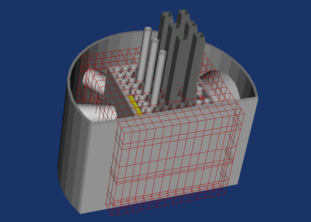
../_images/core_nodal.png — Example of nodalisation for a full MTR reactor model

From the figure you can see that a series of 2D slices are stacked on top of one-another to form a full grid. We will do the same for our simple single assembly reactor.

Building the full-core nodalisation

As described briefly in the previous section, the building of the nodal model is accomplished in two major steps:

The first one is the development of the basic building blocks of the full-core model for all non-loadable (or fixed reflector-type) positions.

Secondly we will add to this additional building blocks for all loadable or moveable components.

Both of these steps will result in sets of of homogenized cross-sections for both the full reactor model and for each loadable component type.

The subsystem within OSCAR-5 used to generate nodal models is named cOMPoSe. There are many levels at which you can interact with the cOMPoSe subsystem. In this tutorial, we will look at the simplest level of interaction which largely automates the construction of the nodal model for you. In later tutorials we will introduce some of the ways in which you can interact with cOMPoSe in a more advanced manner. You will, of course, still have to supply the system with a minimal set of information to set up the nodal model. You will have to:

Select a “primary” core configuration for which you want to generate a nodal model.

Define the radial and axial meshing on which the nodal cross-section generation should take place. This will be accomplished by specifying a 2D radial mesh to define homogenized core components, and 1D axial mesh to define axial cuts.

Specify the parameters that define the reactor states at which homogenized cross-sections should be generated for non-loadable components, as well as boundary conditions.

Build / Select a mini-core configuration for loadable components. These would typically place the loadable component into a representative heterogeneous environment, sometimes referred to as colourset models. This may be as simple as placing a fuel element in an infinite lattice of itself and taking cuts of that model. Remember that loadable components need to be modelled in a representative environment precisely because they will be moved around the core from cycle to cycle, and thus their placement in a given core might not be the ideal representative state.

Specify the additional parameters necessary to generate the loadable component homogenized cross-sections as a function of the reactor state. This means that the loadable component will be calculated at various burn-up levels, temperature and density conditions, since it will experience all of these when later used in the full-core model. A function, which is usually continuous, is fit through these discrete data points to allow cross-sections to be retrieved at other core states in the nodal solver.

Combine cross-sections from Steps 1 to 4, deploy as a nodal core configuration and write all the homogenized cross-sections to a full core library. Each homogenized zone, as defined by the radial and axial meshes, will correspond to a unique cross-section set in the library.

Hint

Remember, a good choice for an axial core cut is one which exhibits only minor axial inhomogeneity over its height.

In our simplified reactor, we have only a single loadable fuel assembly with its own top and bottom structures. Hence point (1) and point (2) will turn out to be identical calculations in this tutorial, although they still represent two distinct conceptually different steps. We will learn more about how to handle the nodal model building for more realistic cases it in the next tutorial. To see how the meshing is done with cOMPoSe, let us open the input file responsible for defining the nodalisation of both the core and the loadable fuel component, located at

<TutorialPath>/SINGLE_MTR_ASSEMBLY/compose/single_mtr_reactor.py.

Remember that we will now use the AutoCompose feature here, which will preset many of the options for you. This file once again has a series of basic definitions at the top (imports mostly). We highlight below only the most important import statement and the first part of the file which defines the full core nodalisation:

from ..configurations.single_assembly_reactor import model

parameters = AutoCompose()
parameters.working_directory = core.utilities.path_relative_to(__file__,'CORE')
parameters.heterogeneous_model = model
parameters.homogenization_grid = \
    [['0' ,'1'],
     ['A' , 1]]
parameters.homogenization_grid_pitches = [[7.71 * units.cm], [8.1 * units.cm]]
parameters.homogenization_axial_mesh = \
   [['TO' , 10 * units.cm],
    ['TI' , 10 * units.cm],
    ['ACT', 59.37 * units.cm],
    ['BI' , 10 * units.cm],
    ['BO' , 10 * units.cm]]

parameters.axial_mesh_bottom = (-59.37 / 2 - 20) * units.cm
parameters.set_state(fuel_temperature = 60 * units.degC,
    moderator_density=LightWater.density_at(40 * units.degC
            ,1.8 * units.bars),
    moderator_temperature=40 * units.degC
                             )
parameters.setBoundaryCondition(boundary_conditions.reflective)
parameters.build_compose_model()

After importing the necessary objects, the core model can be constructed. We start by instantiating an AutoCompose application class and naming the object parameters, then set some data for it. The name parameters is just a local variable name used in this script - you could have called it anything you wish, as long as you consistently update the rest of the script. We typically use parameters for application scripts, since we have to set a number of parameters to define what the script will do. In the above script we:

Set the heterogeneous model as the core configuration (imported at the top), which we built in the previous step.

Define the working directory, where all input files for external codes will be written. This directory is defined here adjacent to the placement of the input, but under a directory called CORE. The name CORE will also be used as the dedicated name for the full-core nodal model later on.

Set the labelled grid and its associated grid sizes to define the radial homogenization mesh. Entries in the homogenization_grid reflect the placement of loadable components. Non-loadable reflectors are denoted as 0, while a non-zero number indicates a type of loadable component. In this case the core contains only a single loadable fuel assembly, so we fill in the grid with a 1. If not specified, it is assumed that the radial homogenization grid is centred at the heterogeneous model centre.

Moving on to the axial mesh structure, define the axial meshing from top to bottom by a series of 2D axial cuts, each with a name, and a size in the homogenization_axial_mesh variable. In this example the, for those with some programming background, is defined as array over the axial height, with each entry in the array given as another array of cut name and size.

Thereafter we place this axial mesh over the model at the appropriate place by setting the axial_mesh_bottom. In this case we have 5 cuts, starting at the absolute position 20 cm below the active core. Remember that the coordinate origin is at the heterogeneous model origin, and unless you chose to override it, it will be in the radial and axial centre of the core. Hence, in this case z=0 would be the axial centreline of the fuel element. You could, of course, have chosen to model a number of cuts over the active height. You would do this if there was a notable axial substructure over the active height of the model. Nevertheless, in this case you have a single active cut (called ACT) and four so-called reflector cuts. The system will determine which type of cut to use automatically. However, you should be aware that reflector cuts are a little special, because you cannot calculate the cut in isolation (with reflective boundary conditions) as you do with active cuts, since then there would be no source of neutrons in the 2D reflector slice. In these cases, the full model is still calculated and used as a driver in order to provide a source of neutrons with the correct neutron spectrum. This then results in a 3D transport calculation as opposed to the 2D transport calculations for active cuts. General Equivalence Theory is not fully applicable to 3D lattice calculations, and thus axial reflector regions will typically not make use of discontinuity factors. This will introduce further differences between the 3D nodal diffusion solution and 3D heterogeneous transport solution, and should be monitored.

Finally you see that we have set the nominal core state to a typical operating hot state in terms of fuel and moderator conditions, defined the core with reflective boundary conditions, and then requested that the compose model is built via the build_compose_model() call.

You can generate the nodalisation visualization yourself to see the cuts that you defined:

>>> oscar5 SINGLE_MTR_ASSEMBLY.compose.single_mtr_assembly CORE visualization

Note here that we choose to visualize the CORE (as defined in your working directory). The reason for having to specify this will soon become evident as we introduce additional loadable components into the script.

After defining the meshing, and setting a few more parameters, the system allows various actions:

We can do the following:

Use the generator mode to calculate these cuts and produce all associated parameters needed to later generate sets of homogenized cross-sections. For this step we will use Serpent.

Use the equivalence mode to post-process the generator mode output and generate cross-sections for a 2D nodal core model (for the cut of interest), and compare the results to the 2D Serpent results.

Use the reconf mode to introduce cross-sections for loadable components in representative environments into the core and determine the accuracy of the approximation of mixing cross-section sets (this one will be covered in the next tutorial).

Use the library mode to generate code specific cross-section files for each homogenization zone, and fit a continuous function through the state points.

Use the deploy mode to generate and save the final nodal configuration.

Use the test mode to perform final 3D testing of the nodal model.

Back to our simple reactor. In order to capture material changes and spectrum effects through the assembly, we define five cuts over the height. One over the active height, two covering the top reflector region, and two covering the bottom reflector region, as per figure below.

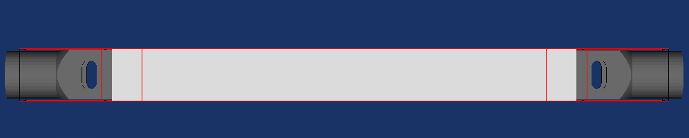
../_images/nodal_model.png — Nodalisation of the fuel assembly

Todo

Visualize the CORE nodalisation and confirm that the nodal meshing is placed as you expect.

Generating and testing 2D cross-sections

Once the cuts are defined, you need to start the process of creating the required set of homogenized cross-sections. The first step is to perform the Serpent calculation to generate the correct tallies from which cross-sections will be extracted. Using the ACT cut as an example, you would typically invoke the generator mode to perform the Serpent calculation via:

>>> oscar5 SINGLE_MTR_ASSEMBLY.compose.single_mtr_assembly CORE ACT generator --config-file buttercup.cfg --target-mode SERPENT execute -- threads 20 --force

This instructs the generator mode to execute a 2D calculation for the active slice from the full-core model. You will note that we choose to use 20 threads here, and add the argument --force to make sure the calculation is repeated and the input file is regenerated, even it if was calculated before. Note that you still have the additional thread control options here as before, such as --peek and --status to see the progress of the calculation. In the next section we will look at how this is done for a loadable assembly in a different colourset environment.

Note that many automation options exist which are not explicitly covered here. For example, the generator mode could also be called without specifying a cut name, in which case all cuts defined in this model would be launched and placed in the server calculational queue. Since these calculations take a little while, we have prepared the output from these runs already, and placed the Serpent result files in the appropriate directory.

It still remains to post-process the results and to check the convergence of appropriate quantities. This is done, for the ACT cut specifically via:

>>> oscar5 SINGLE_MTR_ASSEMBLY.compose.single_mtr_assembly CORE ACT generator --config-file buttercup.cfg --target-mode SERPENT post --show

This action should yield an image such as here. This kind of image shows:

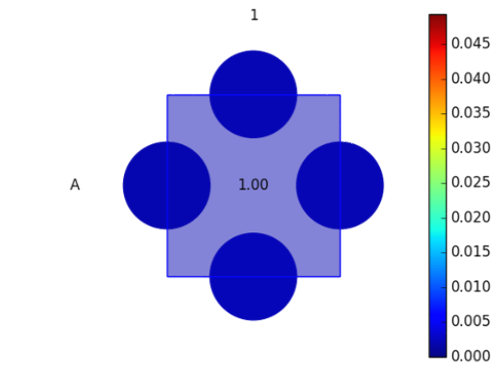
../_images/generator.png — Summary of generator mode errors

A square coloured to show the maximum Monte Carlo error of any nodal cross-section calculated.

A centered text entry showing the quality of a balance check between sources and sinks in the node (ratio printed).

A large circle on every bounding surface showing the level of convergence in nodal currents (needed for calculating discontinuity factors).

A small circle on every bounding surface showing the level of convergence in nodal fluxes (needed for calculating discontinuity factors).

Here we have to make an important point regarding this, and most of the other, tutorials. The post mode reads the Serpent output file, and generates a binary representation of the required data (file with extension .res). We did not add all the Serpent output files to your tutorial sets, as they take a large amount of disk space. We therefore only added the .res files to your tutorials, and therefore you cannot technically perform the post processing. However, as the system will notice that the .res is there and allow you perform the post --show commands. However, if you would add the --force flag to the post processing command, you should expect an error, as the system would not be able to find the Serpent output file in your tutorial set. Once again, the post mode has an option to post process all cuts which were calculated. This would be accomplished via the update mode, by:

>>> oscar5 SINGLE_MTR_ASSEMBLY.compose.single_mtr_assembly CORE update --config-file buttercup.cfg --target-mode SERPENT

Todo

Using the post --show option, make sure that the Monte Carlo calculations achieved sufficient convergence for quantities such as nodeaveraged cross-sections, side-averaged fluxes and currents as well as nodal balance for the ACT cut. After the graphical output is generated, activate the legend and scroll through the results. What level of accuracy would you consider to be sufficient here?

A final important check regarding the cross-sections is now to pass them to the nodal solver and confirm that equivalence between the heterogeneous calculation and nodal solution is maintained. To run the nodal solver for the cut under consideration, and confirm equivalence with regards to reactivity and flux/power distributions, you can call (this of course can only be done for active cuts, as reflector cuts have no sources):

>>> oscar5 SINGLE_MTR_ASSEMBLY.compose.single_mtr_assembly CORE ACT equivalence --errormap

Todo

Perform an equivalence test for the active cut and note the errors in reactivity and fluxes. To what can you attribute these differences?

Adding a loadable component to the core model

Thus far we have constructed the full-core nodalisation, which was only a single assembly. The next step would be to add the loadable components. In this simple case, the only core position is in fact defined as a loadable component (remember the number 1) placed in the homogenization_grid parameter. We now have to define what component and associated homogenization scheme should be applied to loadable component 1. The nodalisation of each loadable component may be done completely independently from the way that the core model was homogenized. You are encouraged to think about the nodalisation of each loadable component on its own. It might very well be that the nodal layer composition of the assembly is the same as that of the core, but this must be decided on a case-by-case basis.

To build the loadable component, we extend the above script with a block of additional parameters to define the loadable component homogenization. See below the extract from single_mtr_reactor.py of loadable component input:

inf_fuel = parameters.create_loadable()
inf_fuel.working_directory = utilities.path_relative_to(__file__,'INF_FUEL')
inf_fuel.colourset_type = InfiniteLattice
inf_fuel.grid_id = 1
inf_fuel.assembly_type = assembly.fueled
inf_fuel.burn_meshes = 8
.....
parameters.build_compose_model()

In the above extract:

We first instantiate a loadable component from the parent parameter class (the call to create_loadable()). By default, this will allow the loadable component to inherit the relevant parameters from the full-core we defined before. The axial meshing scheme and cut definitions, for example, are taken from the parent as a default, but you may decide to override this by re-specifying the axial mesh parameter (thus define inf_fuel.homogenization_axial_mesh here). In this case we choose to simply let this be inherited from the core model.

We again define a working directory, so that calculations for this loadable component will be stored in a dedicated space (in this case then INF_FUEL directory under the compose sub-directory).

We have to choose an environment for the assembly that is representative of the environments it will encounter in the core, as this loadable component will typically be moved to various core positions and its homogenized cross-sections should remain relevant. In this case we choose the InfiniteLattice option, which calculates homogenization parameters for this component in an infinite lattice of itself (reflective boundary conditions). Other options are also possible and will be explored in future tutorials.

We also define to which loadable grid identifier (in this case 1) this assembly is assigned. The grid id refers to entries in your core homogenization grid you defined before in parameters.homogenization_grid. This is an important parameter as both the heterogeneous component model and grid pitches are then automatically extracted from the relevant grid position.

Finally, we defined the assembly type that should be assigned to this loadable component, and choose into how many burnable regions you would like to subdivide the active section of the loadable component.

You could stop at this point and be done with the model. With this subset of the input we could for instance choose to visualise the loadable component via:

>>> oscar5 SINGLE_MTR_ASSEMBLY.compose.single_mtr_assembly INF_FUEL visualization

Notice here that we selected the INF_FUEL model to visualize, as opposed to the previous case where we applied this command to the CORE model.

We could also launch the calculation for all cuts in the loadable component via

>>> oscar5 SINGLE_MTR_ASSEMBLY.compose.single_mtr_assembly INF_FUEL generator --config-file buttercup.cfg --target-mode SERPENT --threads 20

Notice that the generator mode call here is a little different to one before, as we did not specify a specific cut, but chose to let the generator mode calculate all cuts and send their jobs to the server. When complete, we could also auto-post-process all of them via:

>>> oscar5 SINGLE_MTR_ASSEMBLY.compose.single_mtr_assembly INF_FUEL update --config-file buttercup.cfg --target-mode SERPENT

Hint

Whenever repeating calculations that might have been called before, it is often better to add the --force flag to the end of the command, to ensure all old files are overwritten.

This would, however, spawn calculations for all cuts simultaneously, and the matter of resource allocation should be taken into consideration.

If we stopped here, the loadable component would only have cross-sections at a single snapshot, fresh, hot state (if not respecified, the nominal condition for the loadable component is inherited from the core model). We need more, and should additionally:

Specify the possible depletion states of the assembly, by burning it at a typical power and storing cross-sections and number densities as a function of burn-up for later use in the core model.

Specify possible variations in other state conditions (such as fuel temperature, moderator temperature and moderator density) which we expect the loadable component to encounter in the core when used.

We have two options in specifying this additional data:

Import an existing lattice calculational output file from one of the lattice codes coupled to OSCAR-5. You would use this approach when you prefer to set up the lattice calculation by hand and have more control of advanced usage options. In this case you would simply import the lattice output file here and it would contain the burn-up and state dependent cross-sections already calculated. To do this, you would add the following line to your input script:
inf_fuel.external_lattice = utilities.path_relative_to(__file__, '../model/
    lattice/heade/output/FUEL_LEU.HED')
Alternatively, and what we will do in this tutorial, you could generate the lattice parameters for the assembly from this script. This is achieved by specifying a few additional parameters in your input file, and is discussed in the next section.

Todo

Visualize the nodalisation for the loadable INF_FUEL model.

Introducing a lattice cut into the loadable component

As stated above, the input script up to this point will only generate cross-sections for the initial fresh state of the assembly at nominal operating conditions (actually a single set of macroscopic cross-sections per cut). In practical reactor calculations, there are some special requirements for the fuel component cross-sections, as this set of cross-sections should have (as typically calculated by lattice codes):

Fuel cross-sections (in this case the INF-ACT cut) should be generated as a function of state parameters such as burn-up, fuel temperature, moderator temperature and moderator density, so that the core solver can later recover cross-sections for all state conditions of the assembly, as they are encountered. Lattice codes allow for depletion of the cut of interest, as well as variation in other state conditions.

Modern nodal solvers use a microscopic depletion model, meaning that they use primarily microscopic cross-sections from the lattice code (as opposed to macroscopic), and also perform depletion themselves. This is done since the assembly might find itself in a environment quite different from that in which the cross-sections where generated, and so it is more accurate to deplete in the core environment.

Since we choose not to import this additional information from an external lattice calculation, we add some input to the script in order to generate the necessary lattice parameters directly with Serpent.

We will therefore look at some additional cards in the cOMPoSe input for the loadable component, which deals with this data. Consider the following extract from the file:

<TutorialPath>/SINGLE_MTR_ASSEMBLY/compose/single_mtr_assembly.py, that was opened in the previous section:

# Add lattice data to active cuts
inf_fuel.lattice_calculation = True
inf_fuel.pin_cell_mesh = [
[sum([5.150000E-01, 1.900000E-01])] + [1.005000E+00]*6 + [sum([5.150000E-01,
    1.900000E-01])],
    [4.587500E-01] + [4.225000E-01] * 17 + [4.587500E-01] ]
inf_fuel.burn_primitives_in_bundle = AllSeparate
inf_fuel.burn_regions_per_primitive = 6
inf_fuel.burn_steps = \
[0.5,
 1.0,
 3.0,
 5.0,
 10.0]
inf_fuel.state_variation = \
[[state.fuel_temperature      , 60, -30],
 [state.moderator_temperature , 20],
 [state.moderator_density     , -0.193]]

This extract of input sets a few important options:

This input will generate an additional axial cut for each active cut in the loadable component, and prepends the letters LAT- to its name. Thus in this case the new cut created is named LAT-ACT as a special type of cut – a lattice cut. This is as opposed to the ACT cut you defined before, which only extracted a “snapshot” single state cross-section for the material. Now we will burn the material and vary its state to generate multiple sets of cross-section data. We do this to allow the future nodal diffusion calculation to have access to possible states which the assembly might experience.

An overlay pin-cell-mesh is specified as an x-array and then a y-array over the radial dimensions of the fuel plate. This pin-cell mesh is defined for later calculation of intra-assembly power distributions on this mesh, and should relate to the “piece-of-plate” size on which power peaking should be calculated.

The burn-up mesh over the assembly is defined as burning each plate separately (keyword AllSeparate), with 6 equidistant radial meshes over the fuel plate length.

The set of isotopes for microscopic depletion is not explicitly defined here, and thus defaults to a typical set of about 40 isotopes. This can of course be redefined if you wish.

The set of burn-up steps (only 5 in this case) are defined and nominal state conditions are inherited from the core model, since we did not call the set_state routine again for the inf_fuel component.

The set of perturbed state parameters are defined, with deltas of +60°C degrees and -30°C around nominal for fuel temperature, +20°C around nominal for moderator temperature and -0.193 g/cm3 from nominal for moderator density.

Running the cases for the various states of the LAT-ACT cut is done via the following steps:

Firstly, we perform the base depletion of the cut. Currently this will burn the assembly at nominal conditions, but you have the flexibility to have many burn lines if you wish, depending on the nature of the data required by the down-stream fitting codes. The default burn line is called main and we do this via:
>>> oscar5 SINGLE_MTR_ASSEMBLY.compose.single_mtr_assembly INF_FUEL LAT-ACT generator main burn --target-mode SERPENT --config-file buttercup.cfg execute --threads 20
Hereafter (after the run is complete), the result should be post-processed via:
>>> oscar5 SINGLE_MTR_ASSEMBLY.compose.single_mtr_assembly INF_FUEL LAT-ACT generator main burn --target-mode SERPENT --config-file buttercup.cfg post
You can graphically inspect the outcome of the burn line calculation, showing you the evolution of reactivity and number densities during the lattice calculation burn line.
>>> oscar5 SINGLE_MTR_ASSEMBLY.compose.single_mtr_assembly INF_FUEL LAT-ACT generator main burn post --show
Secondly, we have to perform the off-base calculations per burn-step. Although you can choose to launch them at individual burn-up steps, you can also perform all of them at once via:
>>> oscar5 SINGLE_MTR_ASSEMBLY.compose.single_mtr_assembly INF_FUEL LAT-ACT generator main homogenization main --target-mode SERPENT --config-file buttercup.cfg execute
after which the results have to be post-processed again via:
>>> oscar5 SINGLE_MTR_ASSEMBLY.compose.single_mtr_assembly INF_FUEL LAT-ACT generator main homogenization main --target-mode SERPENT --config-file buttercup.cfg post

Notice that the homogenization case was also called main. Multiple homogenization branches are also allowed, which is typically utilized for material off-bases. For example, all state perturbations are required for both the rodded and unrodded state of a intra-assembly control rod. Such examples will be discussed in later tutorials.

Tip

You do not have to perform off-bases at each burn-up step, but select a smaller subset which will still allow a good fit over the lattice data. This is, however, more advanced usage.

Of course we can also perform an equivalence test for the new LAT-ACT cut, by running:

>>> oscar5 SINGLE_MTR_ASSEMBLY.compose.single_mtr_assembly INF_FUEL LAT-ACT equivalence --errormap

Todo

Use the post --show option of the generator mode to visualize the results of the lattice depletion calculation. Can you explain the reactivity trend that you are seeing? What about the evolution of isotopes such as U-235 and Xe-135?

Summary of the AutoCompose generator features

So in summary, you typically would perform these calculations in the following order:

Run and post-process all cuts for the full-core compose model.

Run and post-process all cuts for the each loadable component.

Run and post-process the burn and off-base cases for all lattice cuts.

Todo

Perform an equivalence test for the LAT-ACT cut and note the errors in reactivity and fluxes as compared to the ACT cut. Note this error down for future reference.

The AutoCompose approach to building the nodal model automates a number of things for you. Of course this is useful for typical applications, but there are many more advanced features for customizing the nodal model, and specifically for building the homogenized representation of the core and loadable components in much more ad-hoc ways. In order to see what more advanced usage or interaction with the cOMPoSe sub-system would look like, without the use of AutoCompose, you can browse the following files in the compose subdirectory:

single_assembly_core.py which gives a more detailed compose input file which assumes a little more knowledge of the cOMPoSe application itself, for the full-core model.

fuel_assembly.py similarly gives a more advanced cOMPoSe input file for the loadable fuel element component.

Do not be too concerned to understand these input files now, as we will cover some of their uses in the upcoming tutorials. It is generally suggested that you combine approaches – thus allow AutoCompose to build the base model for you, and then add advanced options as you deem necessary.

Using the library mode

The final action for each cut is to write-out the homogenized cross-sections into so-called HED files (which is the data carrier for few-group homogenized cross-sections), and then to run the POLX code on each HED file. POLX essentially performs a polynomial fit through lattice data. This assists in generating a continuous representation of the originally discreet set of crosssections you have generated (at fixed burn-ups and off-base conditions). The nodal diffusion solver would then be able to query this representation for any state the assembly finds itself in during the full core analysis.

To do this for all the cross-section sets in your model, execute first for the core model:

>>> oscar5 SINGLE_MTR_ASSEMBLY.compose.single_mtr_assembly CORE library --force

and then for the each loadable:

>>> oscar5 SINGLE_MTR_ASSEMBLY.compose.single_mtr_assembly INF_FUEL library --force

and finally do this for the explicit lattice cuts in your loadables:

>>> oscar5 SINGLE_MTR_ASSEMBLY.compose.single_mtr_assembly INF_FUEL LAT-ACT library --force

The --force argument simply reruns POLX even if the output files already exist. You can also run the library mode for each cut separately.

Todo

Run the library mode for all required cuts defined in the previous steps. Do this for the CORE (full core compose model) and the INF_FUEL (loadable) parts of the model.

Deploying the full nodal model

The final step in creating your homogenized model is saving your nodal configuration and generating a single homogenized cross-section library. This is achieved by using the deploy mode. This steps saves the nodal structure of all components back to their assembly archives (the relevant ASM files), and writes up a so-called LNX file, which holds the nodal cross-sections for homogenized materials, to later be read by the nodal solver. You only need to deploy the full core (CORE) model, as it is aware of its loadable constituents. To deploy the model execute:

>>> oscar5 SINGLE_MTR_ASSEMBLY.compose.single_mtr_assembly CORE deploy

Todo

Deploy the nodal model in order to create a LNX file combining all your homogenized mixtures. Confirm after the deployment that the LNX file now exists in your model directory.

Testing the nodal model

We are now ready to test the nodal model. You will see that a basic critical flux test case was defined at the end of the cOMPoSe script. To do this test, we should perform three steps:

Perform the reference 3D Serpent calculation (referred to as reference calculation).

Perform the 3D nodal calculation (referred to as simulator test).

Compare the results.

To perform these tasks, we will now make life a little difficult for you, and suggest that you discover for yourself how to invoke these commands. In this regard the built-in help system is very useful, as you can type any partial command, followed by --help, and your next logical options will be presented to you. Notice that a series of automated test cases where built for you when the nodal model was created. For the purposes of this task, you can use the Critical_case test case.

So beginning with:

>>> oscar5 SINGLE_MTR_ASSEMBLY.compose.single_mtr_assembly CORE test --help

and see if you can proceed through the task below.

Todo

The reference Serpent case has been run for you already. Run the simulator calculation, post-process both results and use the compare mode to see the differences in the results. Note down the errors you discover between the reference and simulator (nodal solver) results, and see if you can explain why they differ.

Step 6: Performing the Nodal Peaking Calculation

We now return to the original problem at hand, and consider the calculation of the power peaking factor in the new assembly design. This is now rather trivial. We repeat the actions we performed to run this calculation in the previous steps, and simply change the target mode from Serpent to MGRAC (the nodal solver), since the model is now created. There is one issue though – you could have generated a number of nodal (compose) models for this reactor, and you have to choose which one to use. If you do not specify, the system will try to make a selection for you, but it is better practice to specify this explicitly. You will note that near the top of you flux_calculation.py script, there is a line commented out, which sets your chosen nodal representation, You must also uncomment this line to tell the system which nodal model you want to use. The nodal model is auto-named during the compose process with a tag taken from the first two characters of your full core nodal model name. In this case it was called CORE, and hence the nodal model is tagged as CO. After uncommenting the line, execute:

>>> oscar5 SINGLE_MTR_ASSEMBLY.projects.flux_calculation --target-mode MGRAC execute --force

Followed by:

>>> oscar5 SINGLE_MTR_ASSEMBLY.projects.flux_calculation --target-mode MGRAC post --show

to have a look at the result. Browse the results and try to see if you understand what you are looking at:

Todo

Execute the nodal calculation and find the maximum peaking position in the assembly and note the maximum peaking factor.

Step 7: Compare the Solutions

To visually compare the results between MGRAC and Serpent, click the icon in the top right-hand corner of the browser to add a results file to the view, and browse to the Serpent results file, which was written during the post mode of the Serpent run. This file is found at:

SINGLE_MTR_ASSEMBLY/projects/SINGLE_ASSEMBLY/SERPENT/plate_powers.res

Todo

Compare the shapes, and consider the different approaches employed in each. Are the results as you expect? Can you explain the different behaviour you see based on your understanding of how the codes approach the problem?