Introduction

Welcome to your first hands-on encounter with the OSCAR-5 system. OSCAR-5 is a reactor calculational platform, supporting a set of different reactor computation codes, focussed on calculational needs for research reactors, power reactors and high temperature reactors. However, the system, and its predecessor OSCAR-4, has an extensive validation basis with regards to research reactor modelling, and the majority of cases considered during this tutorial series will focus on various aspects hereof. This tutorial aims to:

• Acquaint you with the philosophy of OSCAR-5 for reactor modelling, and in particular in the concepts applied in code-independent model building. We will refer to this OSCAR-5 model as the unified model.

• Develop a unified model for a simple reactor (containing only a single fuel assembly), and then deploy that model to both Monte Carlo and deterministic solvers. In this case we will use MCNP and Serpent as Monte Carlo codes, and the OSCAR-4 nodal diffusion package as deterministic code.

• Perform a simple steady state flux calculation and compare the multi-code results. This will help you to understand how the system ensures consistency between high fidelity (Monte Carlo) and operational (deterministic) models and associated solutions.

• Provide you with sufficient background and examples to progress with the remaining set of tutorials.

In this specific tutorial, we will walk through the major steps involved in preparing and executing reactor calculations with OSCAR-5. These steps allow for an extremely powerful feature of using various codes for fit-for-purpose applications, all in a consistent manner. High fidelity codes (such as Serpent or MCNP) can easily accommodate the full heterogeneous reactor details of the OSCAR-5 model, while the development of a homogenized deterministic representation for a nodal solver (such as OSCAR-4) requires a much more advanced approach based on equivalence theory.

Note

Here ‘fit-for-purpose’ refers to the specific combination of accuracy and calculational efficiency most suited to a specific application.

The OSCAR-5 system also features a multi-tier user interface:

• The primary interface level is a script-based system (using Python high-level programming language), allowing the user access to a fairly intuitive reactor calculational framework for building and viewing models, running calculations and post-processing results.

• Further, users of the course can interact with the actual code inputs themselves after they are generated.

• Finally the system has a graphical user interface for controlling the most typical workflow-type activities.

This specific tutorial will introduce the user to the script-based interface, which is the most powerful way to use OSCAR-5, and demonstrate to the user how to calculate a multi-group flux profile through a single fuel assembly in an infinite lattice. In future tutorials, we will expand these concepts to full-core models, and operational calculational requirements such as core-follow and core reload analysis.

For the moment however, let us focus on the joys of instant gratification, and perform our first reactor simulation via a few simple steps.

Background

A detailed heterogeneous reactor specification requires the definition of geometry and material layout of the reactor. In OSCAR-5, such a process is divided into

• building of core components,

• building of core configuration and, finally,

• deployment of this model to a specific code for a given application.

If the model is to be deployed to MCNP or Serpent for a very detailed flux calculation, the specification in OSCAR-5 can generally be faithfully transferred to the target codes. The calculation might take a little while, given the computational cost of these codes, but very little intervention from the user is required after building the heterogeneous model.

However, when we are interested in, for example, performing a large set of core design calculations, it is typical to use a nodal diffusion code for such tasks, since many hundreds (or even thousands) of calculations may be needed, and nodal diffusion codes are highly efficient for such applications. In this case we typically follow a process of spatial homogenization and energy condensation to simplify the model to its final representation. Generally, three steps are involved in these kinds of reactor simulations:

1. The generation of homogenized few-group cross-sections for each of your reactor components, for the appropriate range of conditions (referred to as states) needed during actual full-core simulation. This process implies the definition of a set of state parameters which will be varied to produce homogenized few-group cross-sections for all possible future states of the fuel assembly. We rather calculate all this up-front, and store it for later use, since we do not want to perform transport calculations during day-to-day usage of the model. At that stage, we only want to use the efficient nodal diffusion solver.

2. The set of homogenized cross-sections are fitted in order to produce a continuous representation of the few-group data.

3. The reactor core is assembled from these homogenized materials, and a reactor operational cycle is defined and simulated, allowing the prediction of important reactor parameters like the core multiplication factor k-eff, power distribution and material number densities. This is typically solved with a nodal diffusion method, meaning that relatively large calculational nodes are employed, giving good accuracy of solution on a discretization on the order of a fuel assembly pitch. The module or code used to calculate the nodal diffusion solution on the scale of the full reactor problem is often referred to as the global solver, or alternatively the core simulator. These terms are used interchangeable throughout the tutorial series.

The steps are illustrated below, showing the three steps of single assembly cross-section generation via transport theory, fitting of nodal cross-sections as a function of state parameters, and finally usage of nodal cross-sections in the full-core nodal diffusion calculation. In this example the fuel design and core layout from SAFARI-1 (South Africa Fundamental Atomic Research Installation 1) is used to illustrate the principle.

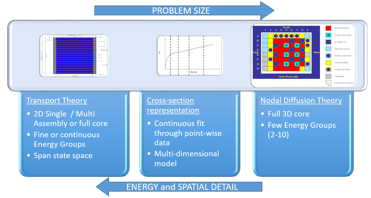
Typical deterministic calculational path

As you can see, these steps are by no means simple and often requires extensive experience in the associated codes and computation methods applied. OSCAR-5 endeavours to simplify this process via a semi-automated process of generating the so-called equivalent nodal diffusion model, in a way that retains as much consistency as is theoretically possible with the original heterogeneous model. The nodal diffusion code within OSCAR-5 is actually an updated version of OSCAR-4.

Hint

To learn more about OSCAR-4 as a stand-alone code, please consult the OSCAR-4 user guides, tutorials and theory manuals.

In this tutorial, we will explore both of these approaches (generating a detailed Monte Carlo and homogenized nodal model) and compare them. Even though the reactor model in this case is relatively simple (just a Material Testing Reactor – MTR – fuel assembly), the concepts and philosophy we will apply is going to remain exactly the same when we move to actual full-core models in later tutorials.

Attention

After this tutorial, you will be able to…

1. Build and view a simple MTR fuel assembly component in OSCAR-5.

2. Define a simple core configuration in OSCAR-5, in this case containing only your fuel assembly.

3. Generate both a heterogeneous Monte Carlo and homogenized nodal model of the core.

4. Perform a simple flux calculation of each and compare the results.

The Scenario

The nuclear engineer in charge of performing reload calculations at your institution informs you that a new assembly type is being considered and a model thereof is needed in order to evaluate its characteristics. You should determine as step one, the reactivity of the fresh element in an infinite lattice of such elements and have a look at the axial power distribution through the assembly. Remember that the assembly has some top and bottom structure and as such an axial power shape will not be flat. Furthermore, as a second consideration, you should evaluate the detailed intra-assembly power distribution in the assembly in its fresh state at the axial layer where the peak power occurs. This will allow you to assess the so-called power peaking factor in the assembly. Consider the various approaches and codes which you could employ to solve this problem, and compare their relevance. A picture of the fuel assembly (plate type MTR assembly design is given below:

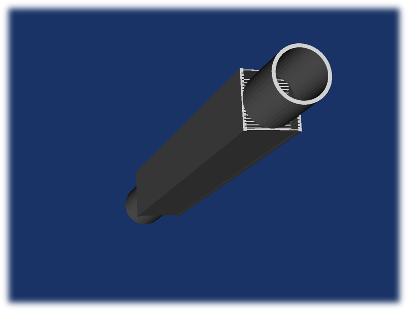
Design of the proposed MTR plate-type fuel design for evaluation

The OSCAR Approach

General philosophy

In the OSCAR-5 code system you have a number of approaches at your disposal to solve such a problem. As “citizens” of OSCAR-5 we have, as part of this tutorial, three options. These are MCNP, Serpent and OSCAR-4. How do we decide how to proceed? Before we make this decision, let us spend some time on understanding the layout of the OSCAR-5 system. which will help to define the options at your disposal.

Note

Remember that OSCAR-4 was only a nodal diffusion package, while OSCAR-5 is a multicode calculational platform which contains its own nodal package as one of the possible targets codes.

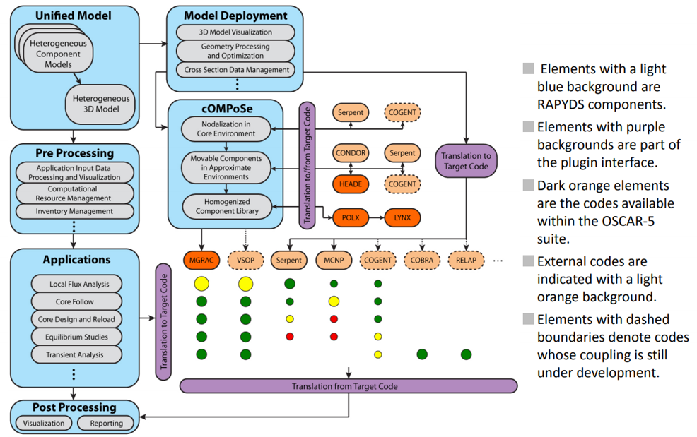
The OSCAR-5 system layout

The structure of the code system is illustrated in the figure above. From the figure, we note:

• The main entry point to the system is the construction of a unified, code-independent system model (top left). A detailed model of each assembly type (including the pool) is built using the Constructive Solid Geometry (CSG) package of the system. Assembly models are combined in an assembly library, from which full-core configurations are constructed. All material properties (isotopic composition and nominal material state, etc.) are also defined in a code-independent fashion.

• Moving from the Unified Model block to the right defines the process of generating the input model for a particular code, including geometry and material specification, while moving down from the unified model definition, describes the path towards generating the application-specific parts of the code input.

• Moving first along the geometry and material specification path, we have:

  1. Support for the model building process, facilitated in the system via extensive visualization schemes, allowing 3D rendering with multiple filters to isolate the components and materials being considered. This can be done at both component and core level. Macros for the automatic creation of typical component types (e.g. plate-type fuel assemblies), geometry processing and mesh optimization schemes as well as mesh completion algorithms all assist in the creation and final deployment of the model.

  2. Translators used to write the geometry and material description of the model to the input for target codes that use detailed geometry. These translators are defined once in the system, and therefore do not depend on the model. This mechanism also ensures that the model remains consistent when it is exported to multiple codes.

  3. The nodal model generator cOMPoSe (which stands for OSCAR Model Preparation System), as detailed assembly and core models cannot be used directly in a nodal diffusion solver. This facilitates the spatial homogenization and energy condensation step. The tool is used to systematically move from the heterogeneous unified description with point-wise cross-section data, to a set of homogenized mixtures with energy condensed to a few-group representation.

• Moving down from the Unified Model description, we have:

  1. A generic inventory management system, which stores the material states of burnable assemblies, makes it possible to use analysis codes lacking this feature for long term core management. It also allows the transfer of assembly states, using a number of options to merge and expand isotopic compositions, to the different codes connected to the system.

  2. Once a suitable model is prepared, it can be deployed to various analysis applications. The figure shows some codes currently coupled to the system, where the dot under each code illustrates the suitability of that code to the intended application. A green dot means the code is perfectly suitable, a yellow dot means it can be used but is not necessarily the best choice, and a red dot indicates that, although possible, the code is not well suited due to feature or resource limitations. The size of the dot indicates the error or level of inaccuracy associated with each code for that application.

The final point above should start to give you some feeling as to the options you can consider for various tasks. For instance, although the nodal diffusion solver OSCAR-4/MGRAC can be used to estimate local flux values in the system, the associated error could be large. The Monte Carlo codes Serpent or MCNP would be much better choices, with MCNP more favourable since it incorporates better estimators in its detector response models. On the other hand, for equilibrium studies where a final core mass distribution is the main outcome, MGRAC will give fairly accurate results in a reasonable amount of computing time, while the Monte Carlo codes will consume many thousands of CPU hours.

Specific deployment strategy for this scenario

So we return to the problem at hand. We are interested in determining some core average parameters such as reactivity and assembly power, but as a second part of the request we need detailed sub-assembly powers. Let us formulate two strategies:

1. Use the system to generate a detailed Monte Carlo model of the system and use it to determine the global, but also local quantities as requested. This will also act as a reference solution.

2. Develop a homogenized nodal diffusion model and use it to determine the reactivity and axial nodal power distribution. We can however go a little further. The nodal methodology does allow for the concept of power reconstruction. This means that even though the solver is intended to generate a solution on an assembly-sized mesh, it does contain a technique for recovering the detailed solution within an assembly. Although approximate, it is instructive to compare this solution to the reference set to determine for which applications such an estimate would be applicable.

Since the generation of the nodal model is quite an important step, we include a little more detail on the process involved in the cOMPoSe subsystem in the next section.

The cOMPoSe philosophy

Moving from a full-detail, heterogeneous model utilizing transport theory for neutronic analysis to a course (or nodal) homogenized representation suitable for diffusion theory is a fairly involved process. There are many factors to take into consideration, but the final outcome would be a model with a limited number of large (assembly-size) nodal meshes, which would allow a very fast calculation of the neutron flux and power distribution, and allow efficient depletion calculations for the core. In order for the model to be useful, it must be prepared in such a way that it captures as much of the neutronic behaviour of the heterogeneous model as possible. In the cOMPoSe system, this typically involves the following steps:

1. For a given core configuration, a coarse radial (or nodal) mesh is chosen, which defines the node sizes. This is typically done in such a way that the fuel pitch is preserved, so that fuelled assemblies fill one node. Next, a number of axial slices are chosen along the height of the model, attempting to limit the amount of axial heterogeneity within a slice. This effectively divides the model into a number of two-dimensional layers stacked upon one-another.

2. Additional nodal meshing must be developed for all loadable components separately. This is typically the case for fuelled assemblies, or any other assemblies that either undergo state changes (e.g. burn-up), or do not stay in a fixed position in the core. This is because, for a fast operational support tool, we do not want to re-homogenize the entire core every time the configuration changes. Thus, fuelled and other loadable assemblies are treated in a more traditional fashion, by performing assembly-level lattice calculations in approximate environments (so-called coloursets). These calculations also account for burn-up and state changes. It is important to note that, since it is difficult to capture all the environments a loadable assembly would experience, this is a typical source of error for nodal methods, and its effect must be carefully monitored.

3. Homogenized cross-sections are then calculated on the nodal mesh for each axial layer, by performing a two-dimensional transport calculation over the entire slice. Generalized equivalence theory (GET) is used to ensure that reaction rates and leakages are preserved for each node. This is done for the full-core model meshed in Step 1 above as well as for each loadable component meshed in Step 2 above.

4. Finally, all two-dimensional layers are stacked together to form a three-dimensional model of the core and a three-dimensional model for each loadable component. Since axial leakage is not preserved via GET, this is another potential source of error and should be monitored.

The process is further summarized in the figure below. The process is shown here for one of the loadable components , but we go through exactly the same process for full core model. In this tutorial of course, the full core is only a single assembly, and therefore the figure applies, in this case, to both the full core and loadables.

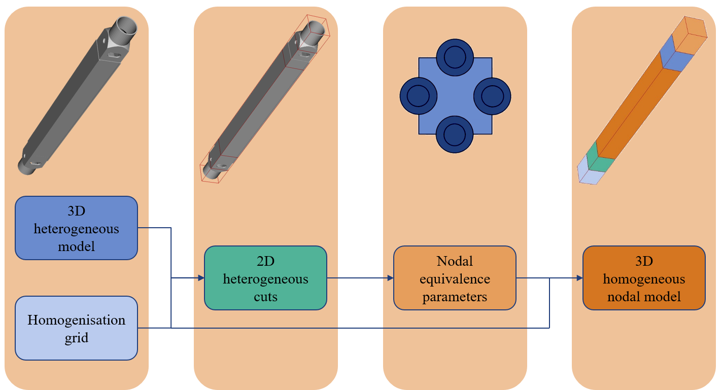
Schematic of the cOMPoSe procedure, for a loadable fuel assembly

During each step of the process, the system gives feedback on the errors (as compared to the detailed heterogeneous model) incurred. Since the errors at the stages of 2D cut generation, lattice replacement and 3D construction are now more traceable, they can be refined, so that one ends up with a nodal diffusion model with acceptable and well quantified errors as compared to the reference heterogeneous model.

Symbols and Abbreviations

CSG Constructive Solid Geometry

cOMPoSe OSCAR Model Preparation System

CPU Central Processing Unit

GET Generalized Equivalence Theory

LEU Low Enriched Uranium

LINX Cross-section library linking code

MCNP Monte Carlo N-Particle Transport Code

MGRAC Multi-Group Reactor Analysis Code

MTR Material Testing Reactor

OSCAR-4 Overall System for the CAlculation of Reactors, generation 4

OSCAR-5 Overall System for the CAlculation of Reactors, generation 5

POLX Polynomial cross-section fitting code

SAFARI-1 South Africa Fundamental Atomic Research Installation 1